New to waves? Here's everything you need to know

Download a PDF of this guide

Download now

1. What really are waves in the ocean?

All bodies of water have waves. These may range from long waves, such as tides (caused by the gravitational force of the Sun and Moon), to tiny wavelets, generated by the wind’s drag on the water surface.

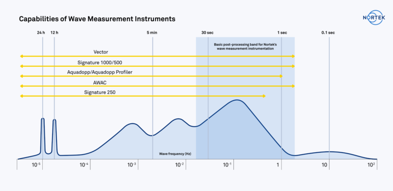
If you were to look at the distribution of energy for waves you would see considerable variability, ranging in period from 12 hours to 0.5 seconds. A significant amount of this energy is found in the 0.5–30-second range – what are commonly referred to as wind waves (see Figure 1). These are the waves that engineers and scientists are primarily interested in when they study wave measurements. The accuracy with which these wind waves can be measured often comes down to which measurement method is used.

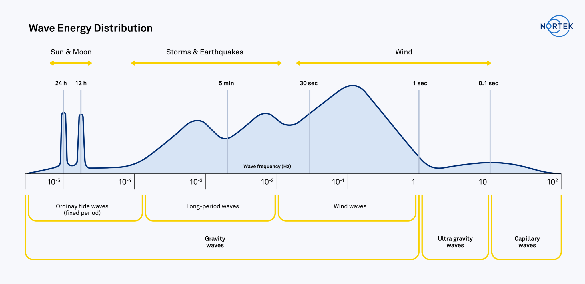
Figure 1: Types of surface waves, showing relationship between the forces that cause them (e.g. wind) and their frequency, in hertz, or period, in seconds (period is the inverse of frequency, so 10 Hz = 1/10 = 0.1 second). The blue shaded area shows the relative energy of each wave frequency. The higher the shaded area, the more energy that frequency has.

This 0.5–30-second band that defines wind waves has variability that makes characterizing waves non-trivial. Waves begin both small in height and short in length, created by local winds, and grow as a function of wind strength, duration of wind and distance. As a result, the wave environment at a particular location may be composed of a combination of local wind waves from a sea breeze and long waves (swell) generated by storms hundreds or thousands of kilometers away.

Therefore, someone trying to measure waves needs to appreciate that the local sea state is composed of waves with different amplitudes, periods and directions. Understanding this is the first step towards making accurate wave measurements.

1.1 How do you measure waves?

Waves are random, and therefore measuring waves requires sampling over a period of time that will best “capture” or represent the complete sea state. As a rough rule of thumb, we try to get 100 cycles of the longest wave we would expect; this means that, if we expect the longest wave period to be 10 seconds for a particular body of water, then 1000 seconds is the preferred sampling length.

The resulting time series of the raw measurements is not particularly useful from a practical standpoint, and therefore needs to be processed to yield parameters that can broadly, yet accurately, characterize the sea state. The most common wave parameters describe height, period and direction of the wave field, and are single values representative of the time series.

1.2 Time-series analysis for wave measurement

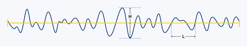
The most intuitive method for estimating wave parameters is to evaluate the time series of sea surface displacement from a single measurement point. A classic example is using a wave staff in a laboratory to provide a trace of the wave’s displacement as it propagates past. The resulting time-series analysis determines how far the water surface extends above and below the mean water level. Individual waves can then be determined by where the trace crosses the mean level and defines the start and stop of the individual waves; this is commonly known as the zero-crossing method (see Figure 2).

Individual waves in the record can then be characterized by period (defined by where they cross the mean water level) and height (defined by the distance from trough to crest between crossings). The result of this exercise is a wave record composed of many waves with a variety of heights and periods.

If these waves are ranked by their height and/or period, then the resulting rankings can be used to calculate common estimates of height and period. Two of the more common estimates are Significant Wave Height (H_s) and Mean Period (T_z). The significant wave height is defined as the mean of the highest one-third of all waves in the record’s ranking. The mean period is the mean of all the periods of the record’s ranking. Other parameters that may be estimated from the record’s ranking are maximum wave height (H_max), which is simply the largest measured wave in the record, and the mean of the largest 10 percent of all waves in the record (H₁₀). The latter two parameters are commonly used for coastal design and assessment and are only possible when we have a direct measure of the surface displacement. Indirect measurements of waves cannot produce these parameters.

Figure 2: Example of a time series of the surface. Here the zero-crossing technique is used to determine individual wave heights (H) and wave periods (L).

1.3 Spectral analysis for wave measurement

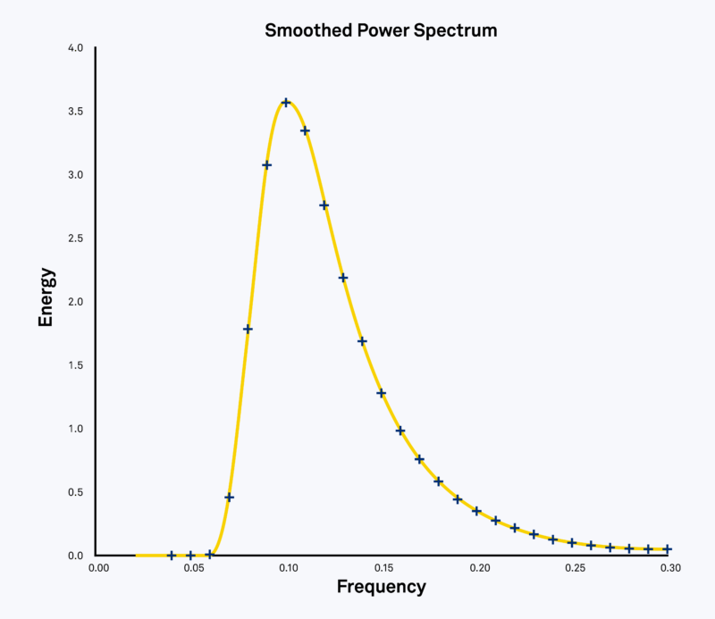
Time-series analysis, as discussed above, may seem like the right way to approach wave measurements, but two common restrictions keep many such analyses from succeeding. The first restriction is that time-series analysis can be a little daunting; the second is that many wave-measuring devices do not have the technology to directly measure surface displacement and, therefore, cannot provide the data needed for time-series analysis. Instead, they measure a wave-related property such as pressure or velocity and infer the sea state from the spectra of the time series (see the example spectrum presented in Figure 3).

The ease of interpretation, together with the wide availability of non-direct measuring instruments, means spectral analysis is the primary method for processing wave results. It provides detailed wave parameters and also permits directional wave analysis.

Wave parameters resulting from spectral analysis include Peak Period, Peak Wave Direction and the spectral analogs of mean period and significant wave height, denoted as T_m02 and H_m0, respectively.

The most complete solution is to carry out both a time-series analysis and spectral analysis. However, this is often not possible with the majority of instrumentation available today.

Figure 3: Energy density spectrum for a time series. This is ultimately used for estimating wave parameters of height and period. Energy is shown in arbitrary units. The important part of the graph is the shape of the curve and the location, along the frequency axis, of where the peak is.

1.4 Subsurface wave properties

Instruments that measure waves from below the surface do so in a variety of ways. The majority measure waves indirectly by a related property, such as the dynamic pressure or orbital velocities.

For those readers not familiar with what happens below the surface when a wave propagates past a point, let us take a moment to explain the basic phenomena.

Figure 4: Description of the wave orbital velocities beneath a wave as it propagates in deep water. Note that the orbital velocity attenuates with depth.

Figure 5: Wave orbital velocities describe different paths as a function of the relative water depth. A wave is said to be a “Deep Water” wave when it is at a depth greater than half its wavelength (> L/2). Its orbital motion is circular and of diminishing diameter with depth (top panel). Conversely, a wave is considered a “Shallow Water” wave when it is at a depth less than 1/20 of its wavelength (< L/20). Its orbital motion is elliptical at the surface and becomes progressively flatter with depth, to the point that, at the bottom, all motion is strictly back and forth (bottom panel). When the wave is at a depth less than L/2 but greater than L/20, it is a “Transitional Wave”. Its orbital motion is elliptical (with a circular form) at the surface and becomes progressively flatter with depth (middle panel).

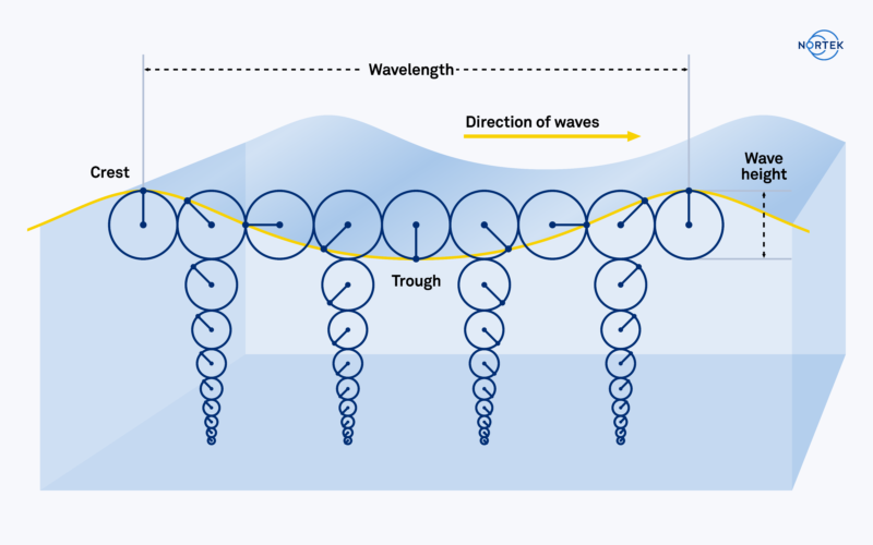
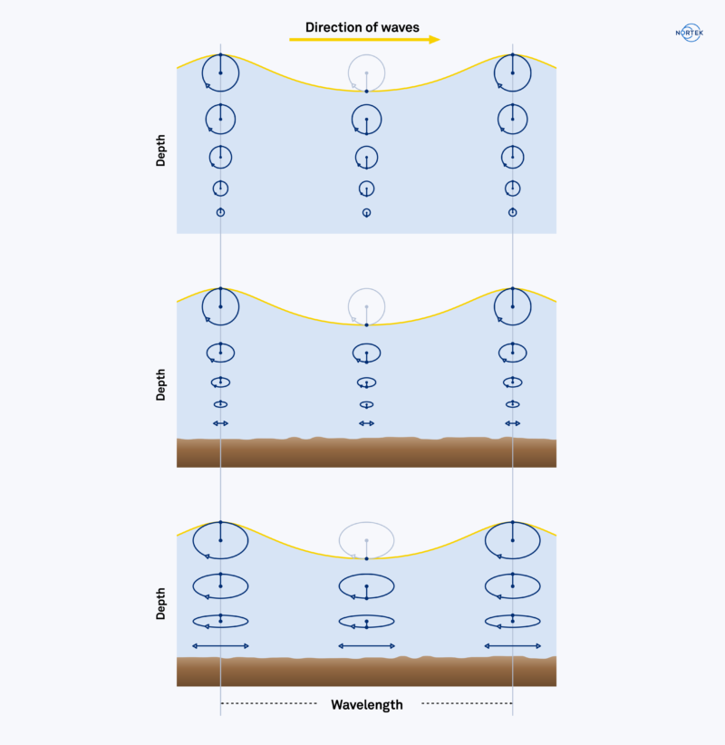
When a wave propagates past a point, it creates local currents below the surface. These currents are special, in the sense that they are changing direction, whereby the affected water below the crest of the wave moves in the direction of propagation, while the affected water below the trough moves in the opposite direction to propagation. This cyclical motion constructs a circular path in deep water and is often referred to as a wave’s orbital velocity.

An important detail to understand about orbital velocities is that they attenuate exponentially with increased depth and shorter wavelength. This means short waves in deep water do not have an orbital velocity signal that penetrates to the bottom. This is similarly true of the dynamic pressure, since it is largely dependent on the presence of orbital velocities, and this means it too experiences attenuation as a function of depth and wavelength.

In the following discussion on measurement techniques, you will see the importance of this and the limits this places on deployment depths as well as the wave types (i.e. long versus short) that can be effectively measured.

Animation showing how wave orbital velocities attenuate with depth.

2. Wave measurement solutions

As a manufacturer of Doppler instruments, Nortek’s wave measurement solutions approach the problem from below the surface. A major advantage of such subsurface measurements is that the instrumentation is located safely below the surface where risk of loss by vessel collision, vandalism or theft is reduced.

A combination of measurements is collected from pressure, velocity and Acoustic Surface Tracking (AST), as we discuss below.

Each of the following methods represents a fundamental improvement over the previous technique, reflecting the evolution over time of the way in which subsurface instrumentation measures waves. The improvement is a result of extending the high-frequency range as we try to best cover the 0.5–30-second waveband.

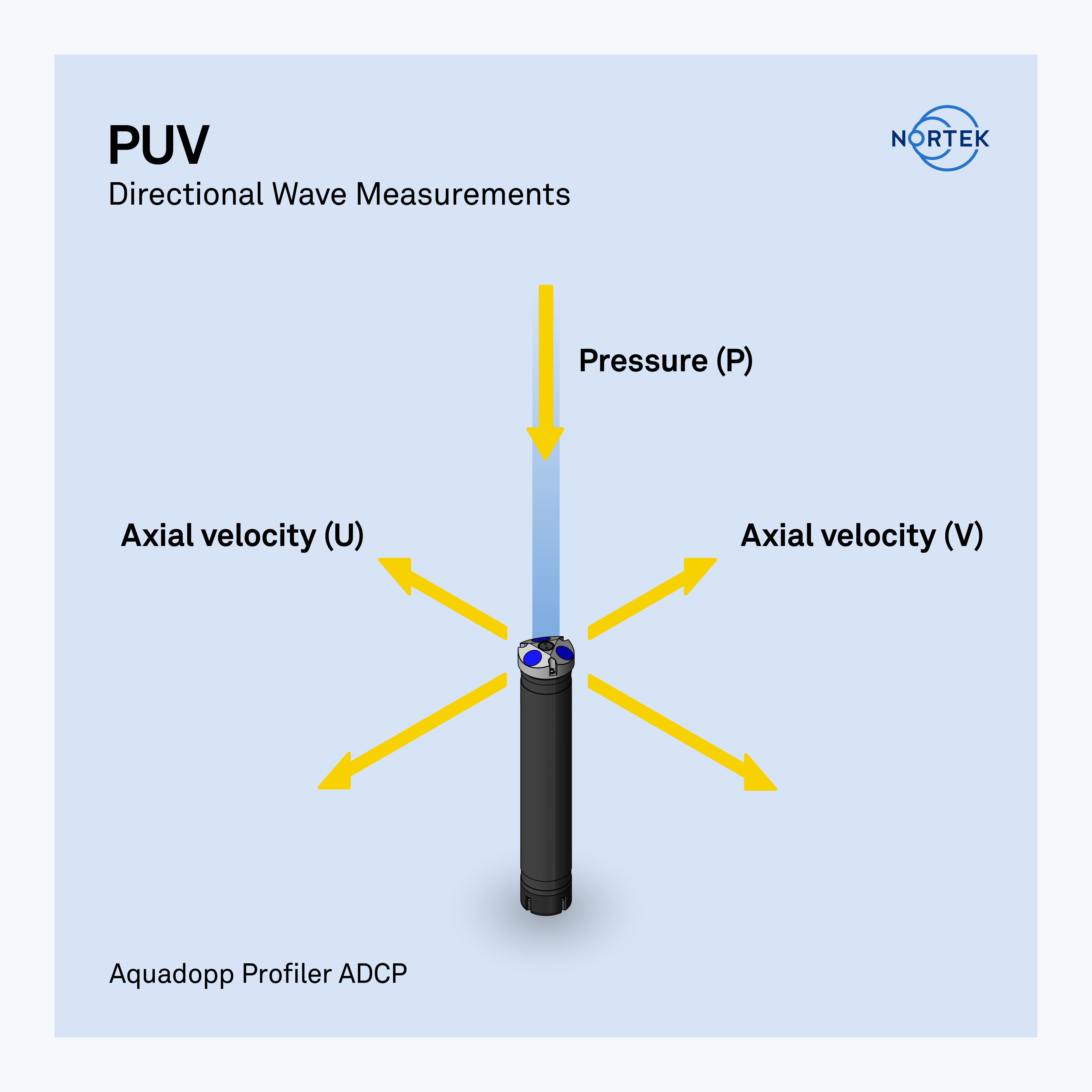
2.1 The PUV method for wave measurement

This method was perhaps the first used for measuring directional and non-directional wave properties from below the surface. It dates back to the 1970s and, because of its modest requirements for instrumentation and processing, is still in use to this day.

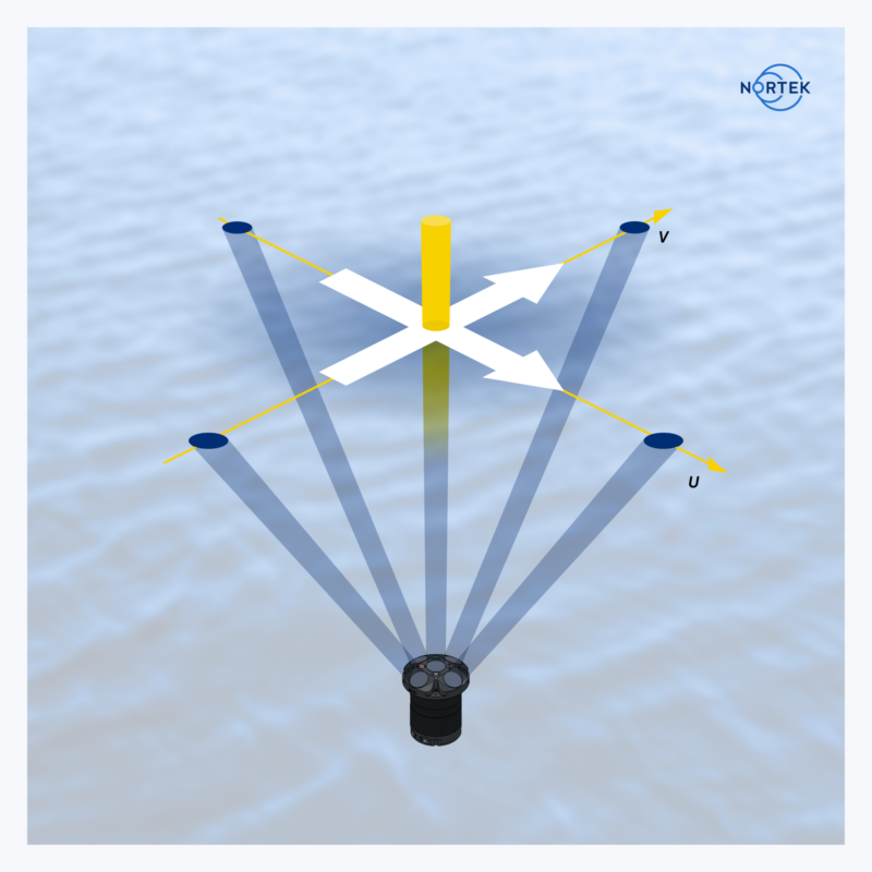
The name itself is a description of the method, as it is an abbreviation of the three quantities measured: Pressure and the two horizontal and axial components of the wave’s orbital velocity, U and V. The pressure measurement provides a means of estimating all the non-directional wave parameters, and the combined P, U and V measurements allow for estimating the directional wave parameters. These measurements are made at the instrument’s deployment depth, and because they are located at the same point, this is referred to as a “triplet” measurement.

Download PDF version of this guide

An important detail to understand about orbital velocities is that they attenuate exponentially with increased depth and shorter wavelength. This means short waves in deep water do not have an orbital velocity signal that penetrates to the bottom. This is similarly true of the dynamic pressure, since it is largely dependent on the presence of orbital velocities, and this means it too experiences attenuation as a function of depth and wavelength.

In the following discussion on measurement techniques, you will see the importance of this and the limits this places on deployment depths as well as the wave types (i.e. long versus short) that can be effectively measured.

Animation showing the impact of passing waves on the pressure and velocity detected by a sensor on the seabed. Note that for simplicity, no differentiation is made between hydrostatic pressure (i.e. the pressure induced purely by the height of the water column above the seabed) and dynamic pressure, which is heavily dependent on the presence of wave orbitals.

Nortek offers three instruments for PUV measurements. These are the Vector, the Aquadopp Current Meter and the Aquadopp Current Profiler.

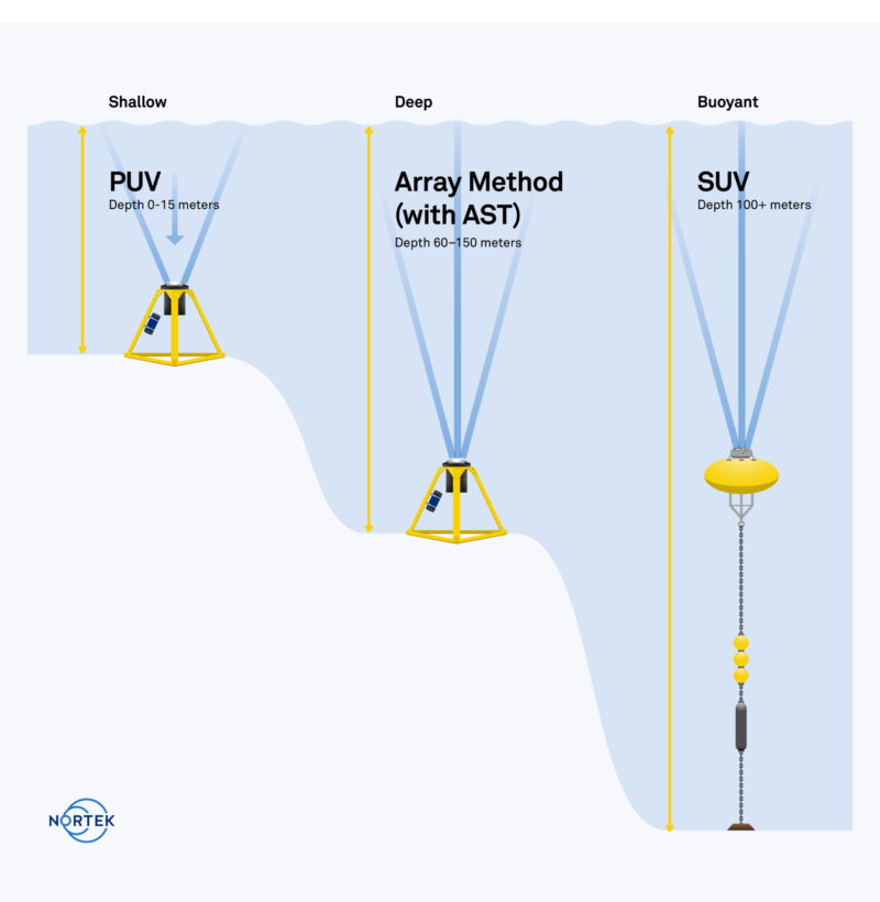
The most important thing to understand about the PUV method is that it is limited to (a) deployment depths that are shallow (less than 10–15 m) and (b) waves that are long (periods of approximately 4 seconds or longer). The limitation of only measuring long waves (swell) is the one that should raise a warning flag for those who are interested in the complete description of the wave environment.

Nortek Aquadopp Profiler ADCP and the PUV method — Figure 6: General schematic of a Nortek Aquadopp Profiler ADCP showing orientation of horizontal velocity (U and V) and pressure components (P) that together make up the PUV method.

As discussed above, the accuracy of the solution requires measurements over the entire wind-wave band (0.5–30 seconds). Incomplete coverage of the wind-wave band can result in underestimation of wave height and missing peaks in the spectrum. The only way to improve the coverage of the wind-wave band is to deploy the instrument in relatively shallow water (i.e. 3 m depth).

The reason why the PUV measurement method cuts off at some given period is that the signals that are being measured (pressure and orbital velocity) have a dramatic attenuation that is a function of both deployment depth and wave frequency (period).

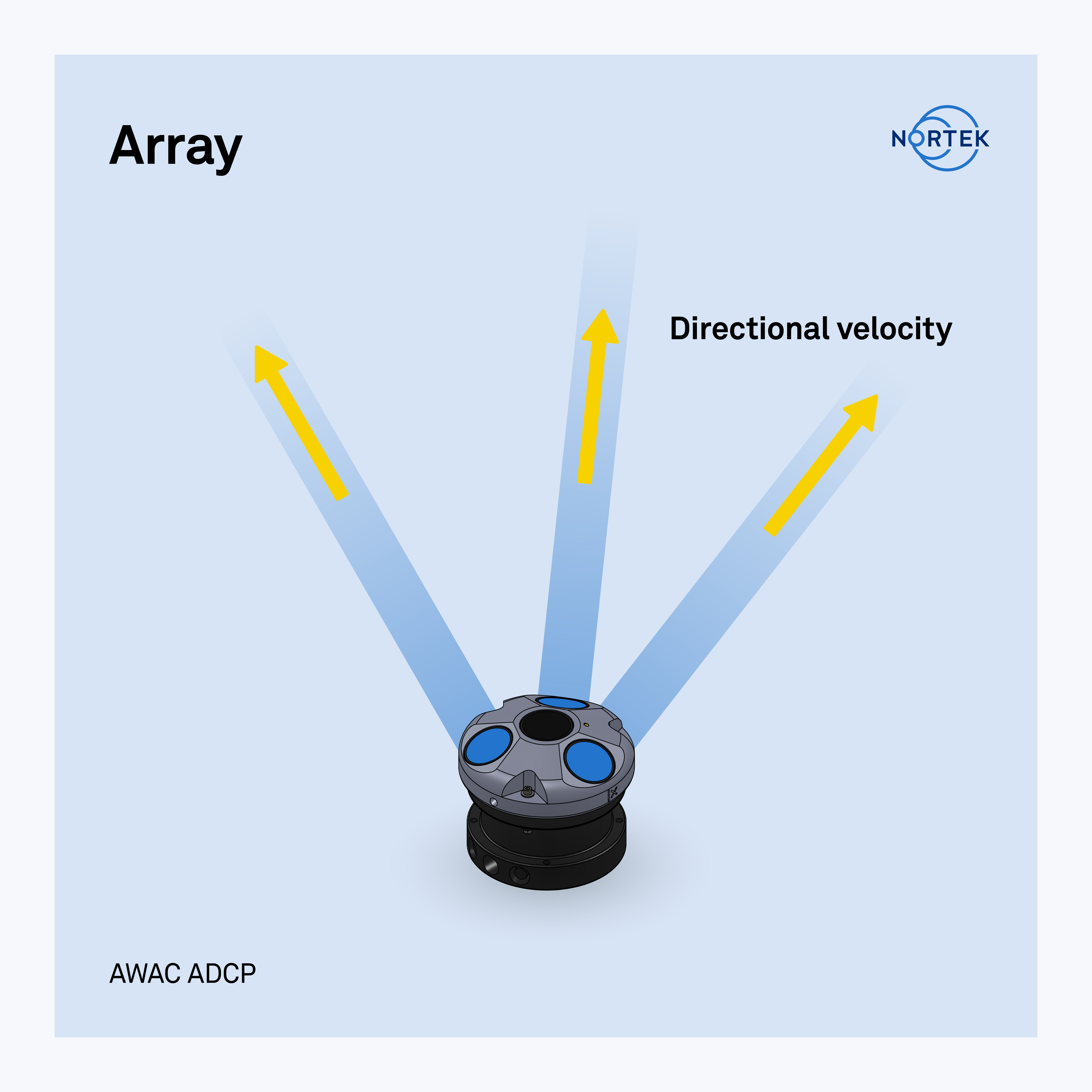
2.2 The array method for wave measurement

The shortcomings of PUV instruments prompted the development of a new technique for measuring waves in the early 1990s. This involves employing current profilers to measure orbital velocities closer to the surface where the orbital velocities are less attenuated by depth. As a result, the shorter waves can be measured at greater depths. This leads to an effective doubling of performance; the deployment depth could be doubled, or the cut-off period was reduced by half.

This method, however, is not without its shortcomings. More complex processing is required, since the measurements are no longer collocated, but are in the formation of an array of measurement cells below the surface. The most common array processing method is the Maximum Likelihood Method. The solution is non-trivial; this means it lacks the “do it yourself” option for processing. Nonetheless, the method has demonstrated very favorable results.

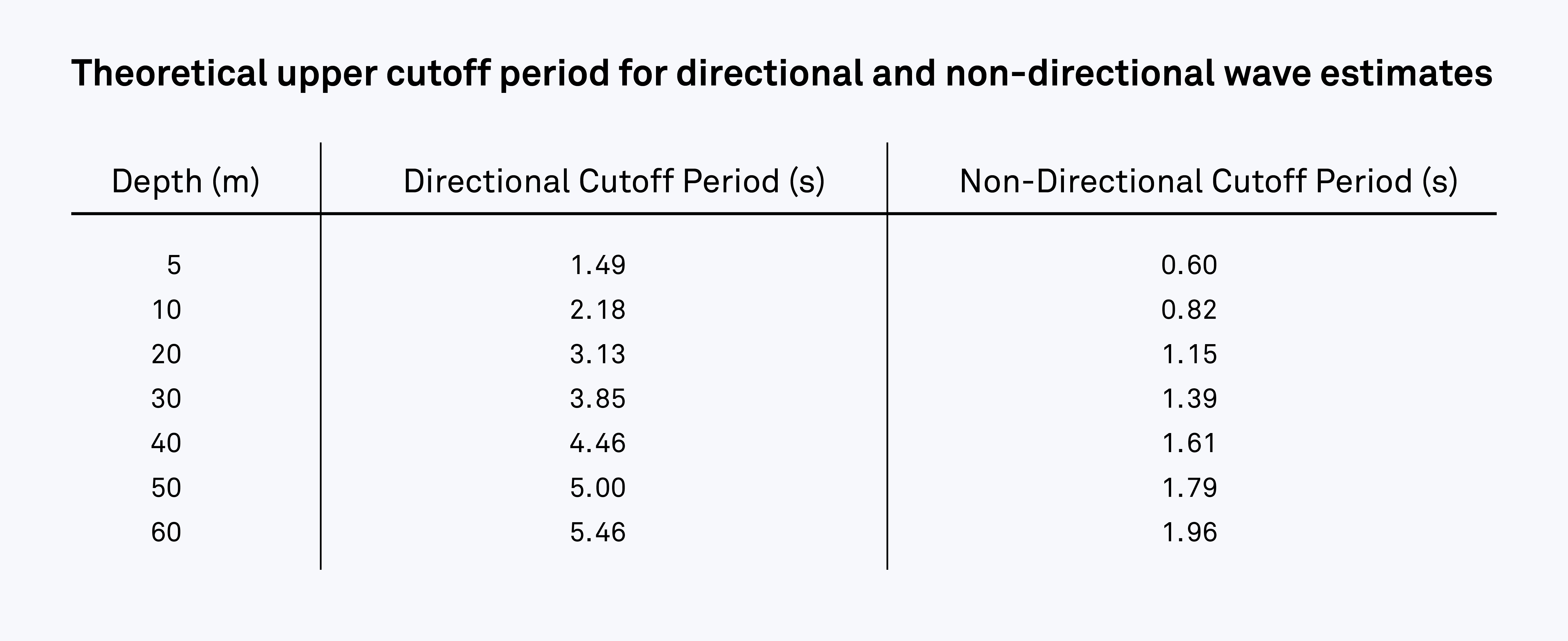
The important detail about the array solution is that the complete wind-wave band (0.5–30 seconds) is still not covered and underestimation is possible if the instrument is deployed in typical coastal depths (e.g. greater than 15 m). The limitation is a result of the horizontal spacing of the velocity cells that construct the array near the surface. When the spacing is greater than half of the wavelength that is being measured, the solution is no longer valid. Furthermore, this limitation is imposed on both the directional and non-directional solution. Table 1 below indicates the expected cut-off periods for various depths.

Nortek’s standard AWAC offers this solution and reduces the limitations imposed by the PUV method by a factor of two. This solution was a large step forward for subsurface wave measurements, but the complete wind-wave band still needed to be resolved in order to avoid underestimating wave height. This led to more direct measurements of the surface.

New to waves Fig New1 B 001 rev02 — Figure 7: General schematic of a Nortek AWAC, showing orientation of velocity beams used in the Array method. This allows wave orbital velocities to be measured higher up in the water column (closer to the water surface) where the wave orbital velocities are less attenuated. Note, however, that the farther you are from the instrument, the greater the distance between each acoustic beam.

Theoretical upper cutoff period, in seconds, for directional and non-directional waves — Table 1: Theoretical upper cut-off period, in seconds, for directional and non-directional waves.

2.3 Acoustic Surface Tracking (AST) for wave measurement

In 2002, the AWAC was first released with the Acoustic Surface Tracking option. The vertically oriented transducer in the center of the AWAC could now be used to measure the distance to the sea surface directly by using the simple echosounder principle. The direct measurement (as discussed earlier) has many advantages; the first, and most profound, is that there is effectively no depth limit for coastal waters and that the largest possible portion of the wind-wave band is covered. The AST measurement also allows for both time-series and spectral analysis. This means design parameters such as H₁₀ and H_max can be measured directly.

Figure 8: Location of the center beam on an AWAC, showing the Acoustic Surface Tracking (AST) principle where distance to the sea surface is measured with an acoustic sensor.

Since the inception of the AST, it has remained the cornerstone of the success of the AWAC. Numerous comparisons have been made with independent and trusted references; the data return has always been near 100 percent and the estimates of the wave parameters very favorable. In short, the AST circumvented all the shortcomings associated with subsurface wave measurement instruments and allows for the best possible coverage of the wind-wave band.

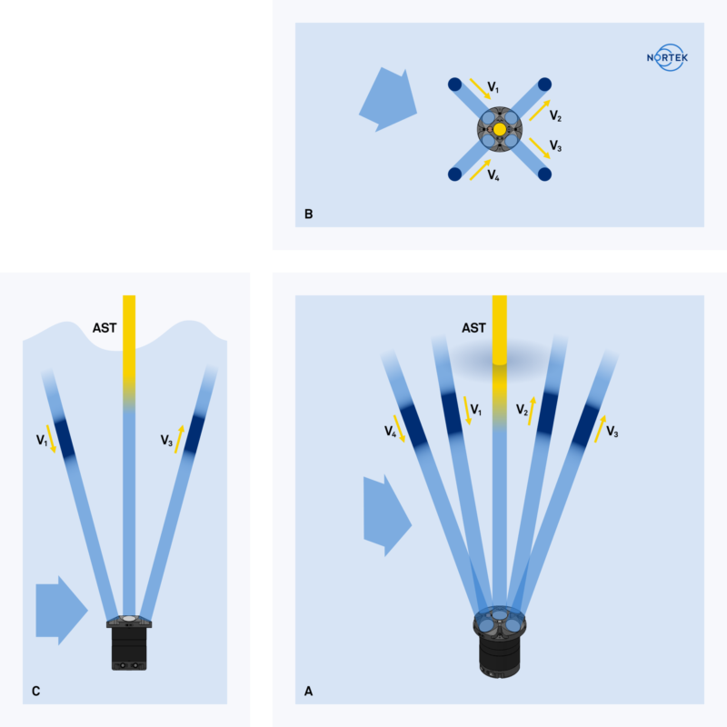
2.4 Directional wave measurements with AST

The AST measurement by itself was limited to improving only non-directional wave estimates. This meant that the array method was still used for all directional estimates and therefore limited to the depth-dependent array size.

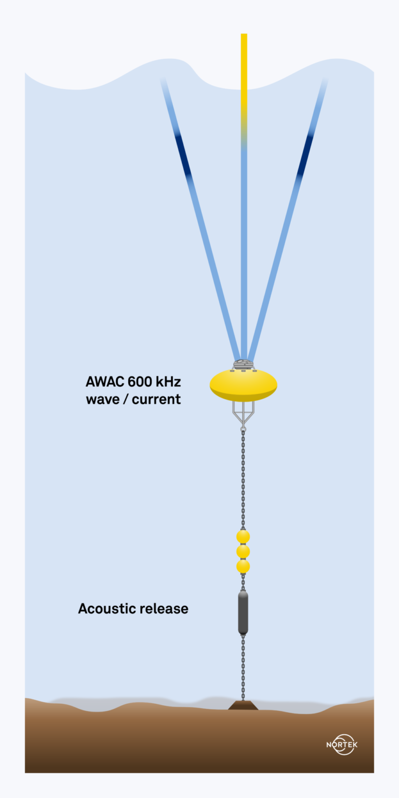
In 2005, Nortek patented a new method for processing wave data from the AWAC with AST, called the SUV method. The solution represents a hybrid of the PUV and AST measurements. Wave orbital-velocity measurements are still made close to the surface, like the array solution, but instead of using an array, the velocities are converted to the axial velocity components of U and V. The other difference is that pressure is no longer used, and the AST is used in its place (surface measurements, S).

Figure 9: Location of measurement cell array for orbital velocity measurements (dark blue) and Acoustic Surface Tracking (yellow). Figure A is an oblique view of all four slanted beams of a Nortek Signature 500 (used for velocity measurement) plus the center beam (used for AST measurement). Figure B is the same as A but viewed from above. Figure C is the same as A but viewed from the side. The extent of the cells in the array (dark blue sections along each slanted beam) are shown shorter than they truly are for easier viewing. The large, light-blue arrow represents the current direction.

The result is a solution that permits the AWAC and any Nortek ADCP with a vertical beam (e.g. most of the Signature ADCPs) to be mounted on the bottom or, as not traditionally possible, on a subsurface buoy. This means that when wave measurements are desired in waters where it is not possible to use the array solution (60–100 m deep), the instrument may be placed on a subsurface buoy and positioned closer to the surface (e.g. 30 m below the surface). The SUV method accounts for and corrects for the rotation of the buoy, making these measurements possible.

The instrument measures directional wave characteristics as if it were mounted on the seabed at 30 m, yet it has the flexibility to be mounted at depths determined by the subsurface buoy’s mooring system.

Figure 10: Directional measurements with AST. Here an AWAC 600 kHz ADCP is shown deployed on a subsurface buoy and positioned close to the surface.

Figure 11: Directional wave measurements with AST. Image shows location where both the slanted beams as well as the center AST beam intersect the water surface.

2.5 Summary of wave measurement methods

Hopefully, this discussion has helped to illustrate the differences between the measurement methods and the limitations of each. In the end, the accuracy of the estimate is, to a large extent, dependent on how well the wind-wave band is measured. The method that is ultimately chosen should reflect the measurement objectives in terms of how much of the waveband needs to be represented.

Figure 12: Each of the three wave measurement methods available from Nortek – PUV, the Array Method (with AST), and SUV – allows users to place their systems at practically any depth.

The PUV instruments are fine as long as the water depths are shallow and only the long waves are of interest. As an example, the PUV may be successfully used if one wants to investigate a structure’s response only to swell in shallow water. However, there would be a risk of underestimating wave height if one wanted to measure the complete wave environment some distance seaward of a harbor entrance.

Experience has shown that there are almost no users who use a standard AWAC ADCP without the AST. A pure array solution of just velocity measurements is simply too limiting when the option of including the AST measurement is easily included. The value and flexibility that the AST provides mean that users tend to evaluate between a PUV solution and the AWAC with AST. PUV measurements tend to be specific to special projects, and one must consider the deployment depth and wave frequency of interest. End users evaluating the most cost-effective option are encouraged to discuss the possibilities with a Nortek associate.