Revealing complex tidal flows in the Santos Estuary with a vessel-mounted ADCP

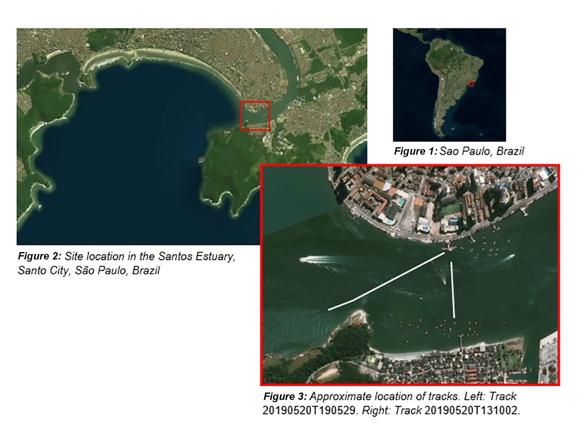
The Santos Estuary, on the coast of central São Paulo state, is a tidal estuary bounded by two channels that discharge into the Bay of Santos. This made it a good location for a Nortek team to demonstrate how ADCPs can reveal complex current movements.

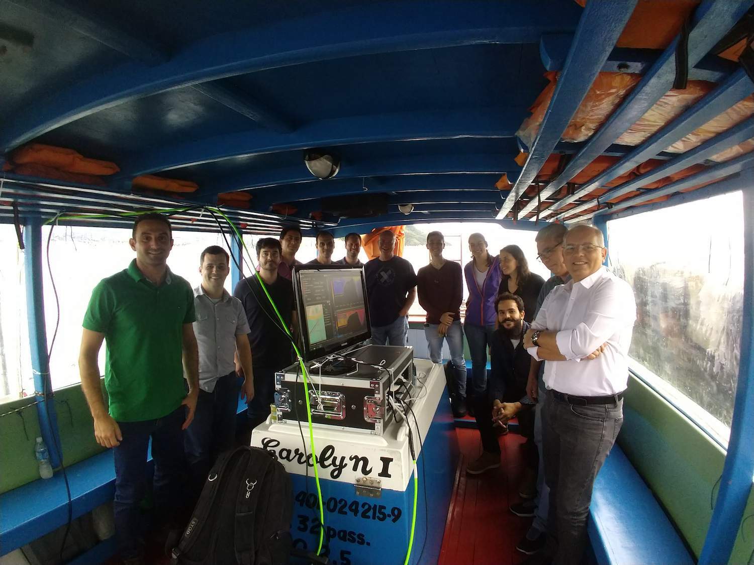
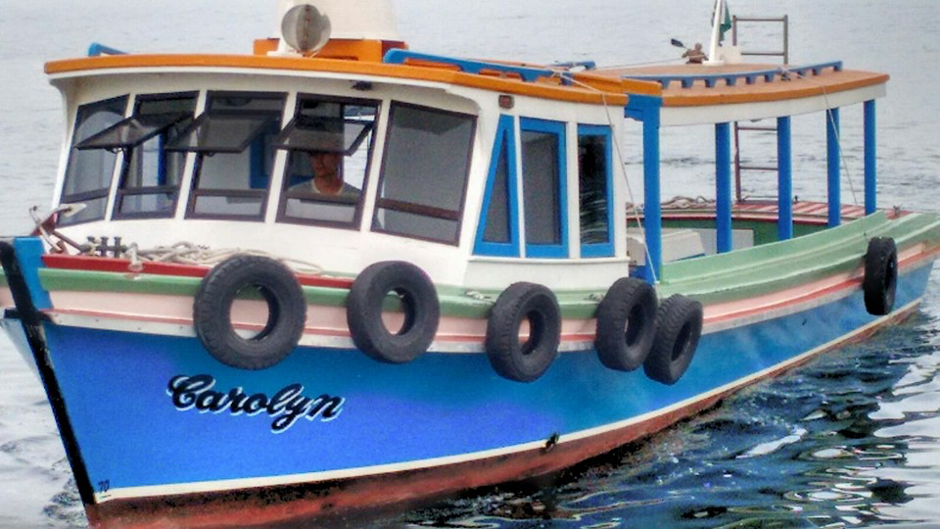
The team used the Signature VM Coastal, fitted with a Signature 500 ADCP to the vessel Carolyn, and then sailed along two transects across the estuary.

The demonstration provided plenty of food for thought for the observers, with the results providing interesting illustrations of how tides act on water in the estuary. The 500 kHz ADCP recorded profiles using 0.5 m cells, with a sampling rate of 1 Hz.

Creating a cross-sectional current profile of the estuary during flood tide

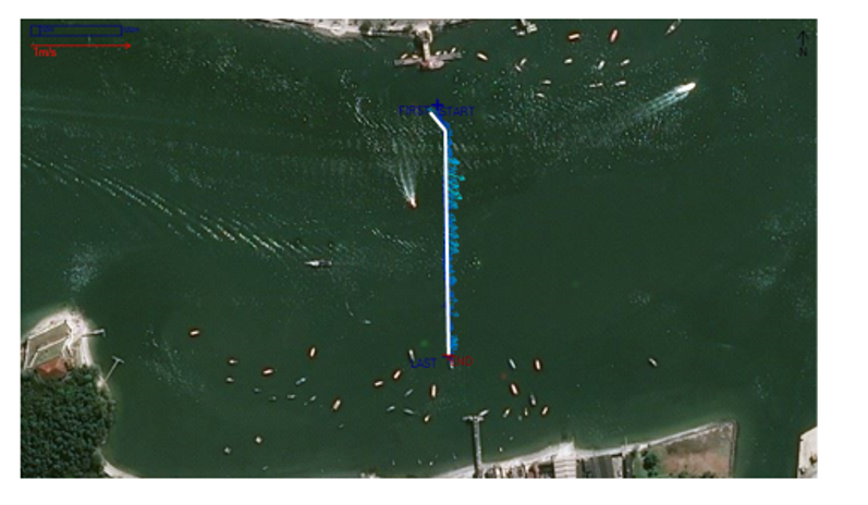
The first transect (track 20190520T131002) extended approximately 300 m across the channel, roughly perpendicular to the banks. The deployment took place as the tide migrated landward into the estuary.

The ensemble of measurements taken by the Signature 500 as the vessel sailed along this transect – a trip that took just a couple of minutes – creates a cross-sectional profile of the estuary.

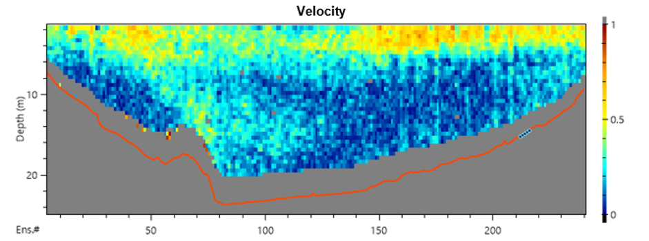
Figure 4 indicates the average flow velocity recorded by the Signature 500 across the water depths measured, which extends down towards 20 m (flow is volume per unit time). These average velocities are small, just a few tens of centimeters per second at their greatest, towards the north end of the transect.

However, a closer look at the data, processed using Nortek’s Signature VM Review software, reveals a more nuanced picture.

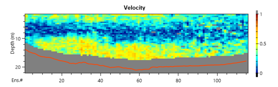
Figure 5 shows the velocity of the water at different depths across the transect. The near-stationary water at mid-depth (the blue band) resides between surface and bottom layers with velocities as high as 0.60 and 0.75 m/s, respectively.

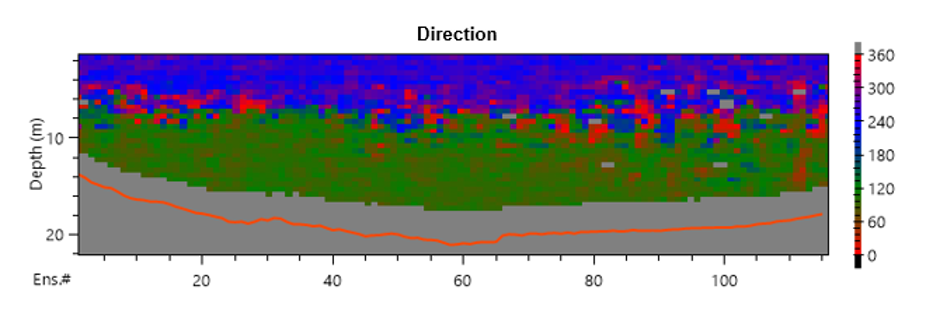
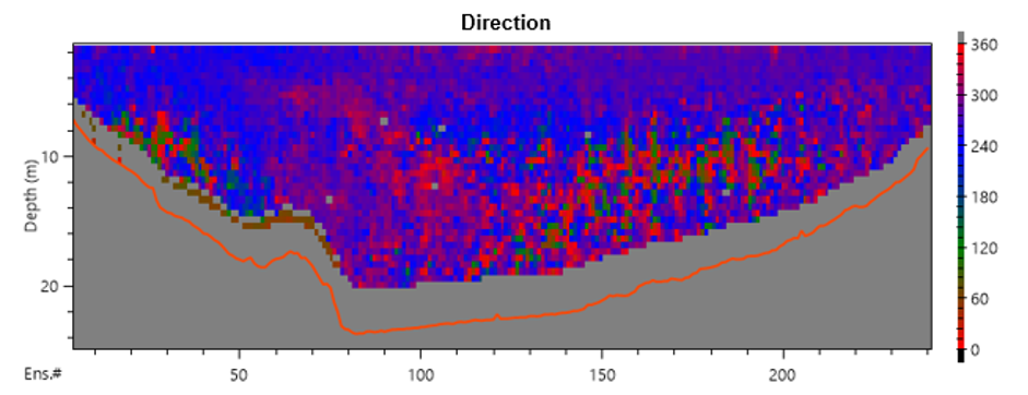
More of the picture is revealed in Figure 6. This directional data shows seaward flow in the upper layer, where more buoyant water typically resides. Landward flow in the bottom region suggests tidal inflow. A transitional layer is visible in the middle.

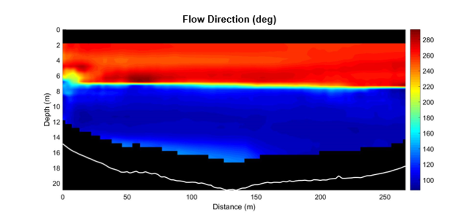
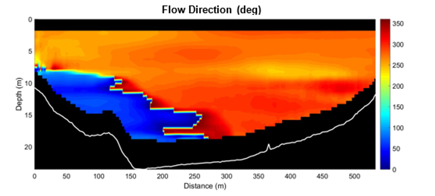
The tidal and freshwater forcing are visualized dramatically in Figures 7–9. Here, data have been processed with the United States Geological Survey software package Velocity Mapping Toolbox (VMT), which typically uses longer averaging times to produce smoother images.

The VMT-generated flow direction plot (Figure 7) shows distinct upper and lower regions and a narrow transitional band at 6–8 m depth.

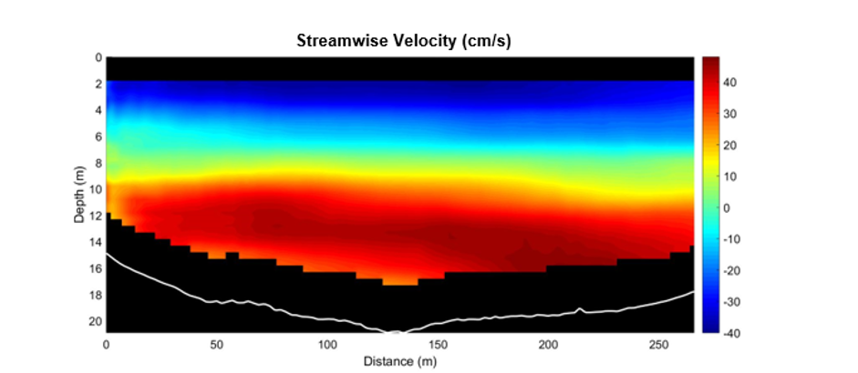
The streamwise velocity plot (Figure 8) also shows three regions, with the largest values at the surface and in the center of the bottom layer. The lowest velocity is in the transitional band at a depth of approximately 8 m.

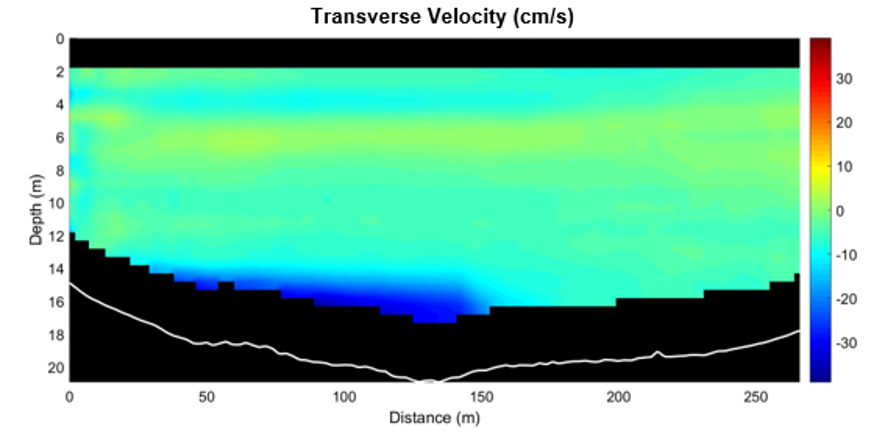
A VMT-generated transverse velocity plot (Figure 9) shows that, overall, the transverse flow in the channel is weak and uniform, with a dominant region at the bottom.

Creating a cross-sectional current profile of the estuary during ebb tide

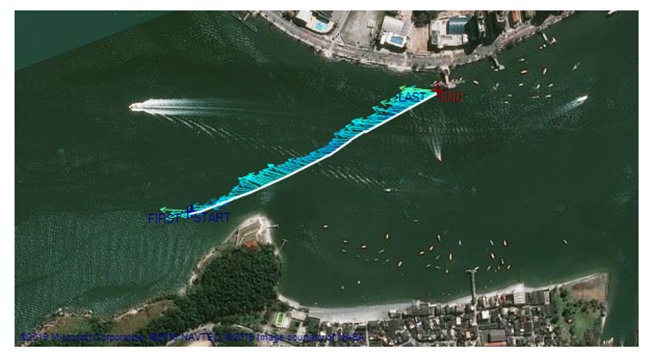
The second track (20190520T190529), skewed across the channel around a headland, was deployed around six hours later during ebb tide. This track reveals a very different picture.

Downstream flows are stronger overall, as Figures 10–12 show. Velocity is generally strongest at the surface, where seaward flow has minimal friction and decreases towards the bed. The direction plot depicts a dominant seaward current at the surface, with a weaker landward, tidal component in the lower half.

The image obtained using VMT processing (Figure 13) clearly shows the predominant flow direction out to sea.

Efficiency in producing current profiles for a complex area

This demonstration encapsulates what can be achieved in just a short period of time to produce current profiles for a complex area such as a tidal estuary.

A full survey of this type typically involves carrying out perhaps 20–30 passes along a given route across a 13-hour tidal cycle, providing highly detailed data for analysis. But the principle is the same, and with the right equipment, this can be a relatively straightforward process.

Creating a meeting place for users and experts

Around 20 Nortek customers and potential customers from Brazilian academic institutions, industry and government bodies were on board to watch the demonstration.

“There were people seeking to improve their use of instruments in research, those who want to use our instruments to provide services to other companies, and potential new users, including oil companies, getting to know the latest technologies,” says Diego Bitencourt, Director of Nortek Brasil, who organized the event.

“It was good to have a lot of users and experts in the same place to meet and share information. They don’t get many opportunities to do that otherwise,” he adds.