Understanding ADCPs: a guide to measuring currents, waves & turbulence with acoustic sensors

1. Introducing Doppler technology and ADCPs

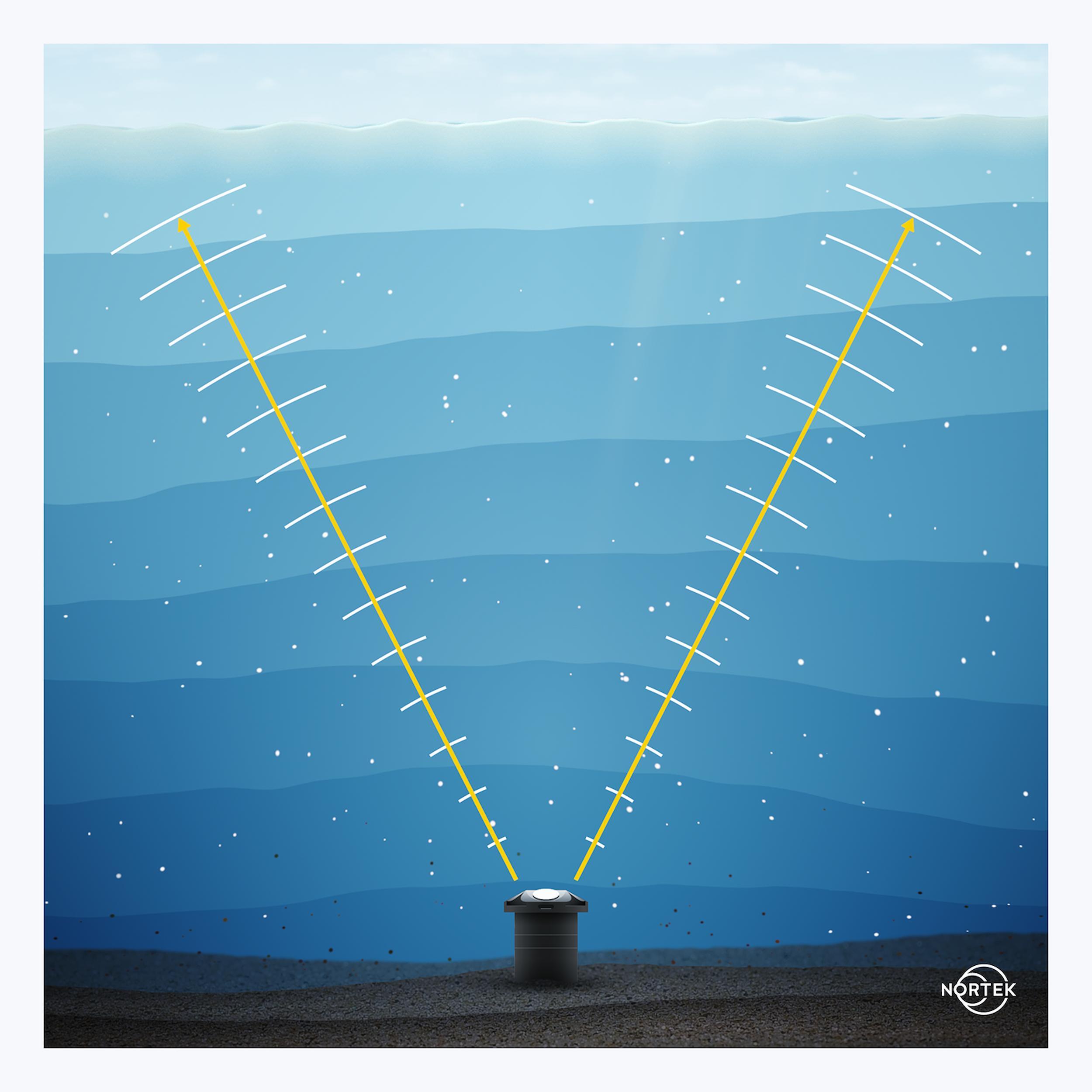
ADCPs are instruments that measure water velocity by using underwater acoustic technology. In a similar way to sonars, ADCPs transmit acoustic signals that propagate through the water column, away from the instrument. These signals reflect off particles in the water, producing echoes that are detected back at the ADCP. The ADCP can then build a velocity profile from these echoes by slicing the water column into multiple layers, measuring the velocity inside each layer. This is conceptually illustrated in the video below.

ADCPs have now been with us for 40 years. They started out measuring current profiles in the ocean, and they have since been adapted to a wide range of applications, including waves, turbulence and subsea navigation. All of these applications are affected by the principles outlined in this guide. Although this guide primarily addresses ADCPs, the principles also apply to other Doppler instrumentation, including single-point current meters, velocimeters and Doppler Velocity Logs (DVLs).

Although the earliest ADCPs date back to the early 1970s, they didn’t become commercially available until the early 1980s, when a company called Rowe-Deines Instruments launched the earliest successful commercial current profilers. Since then, ADCPs have undergone amazing development and transformation. They were difficult to use at first: in the early days, ADCP users had to spend a lot of time learning about the technology so that they could get the data they wanted and to ensure the data quality was good enough to use.

Engineers have worked hard over the years to perfect the operation of ADCPs and to make them easy to use. They have since become so good and the accompanying tools so useful that you can focus on your science or engineering without having to think so much about the details of the instruments you are using.

ADCPs are just one of many sensor types that measure water velocity, but they have become the most commonly used sensor for oceans and inland waters because they make it so easy for users to get top-quality data.

2. The Doppler effect

The Doppler effect is named after 19th-century Austrian physicist Christian Doppler, who used it to explain the color of light coming from binary stars. To demonstrate how it worked, he placed trumpeters in an open carriage on a train and had musicians standing next to the train tracks listen to the pitch of the trumpets as the train moved back and forth past them. This introduces us to two key concepts in acoustics: source and receiver. In this illustration, the trumpets were the source of the sound, while the listening musicians were the receiver of the sound.

One example we can use to illustrate the Doppler effect is that of the sound of the engine of a racing car. The sound of the car’s engine changes pitch in a familiar way, due to the Doppler effect. The pitch is higher on the approach and lower as the car moves away.

This animated video of a racing car’s engine as it passes by illustrates the relationship between frequency and travel time. If you are in front of a moving car, the second wave takes less time to get to you than the first wave, because the car’s velocity has moved it closer to you. In front of the car, the travel time gets less and less and the pitch goes up. Behind the car, the travel time goes up so the pitch goes down. If you know one, you can compute the other.

This is relevant to ADCPs because they nearly always measure changes in travel time to determine the Doppler effect.

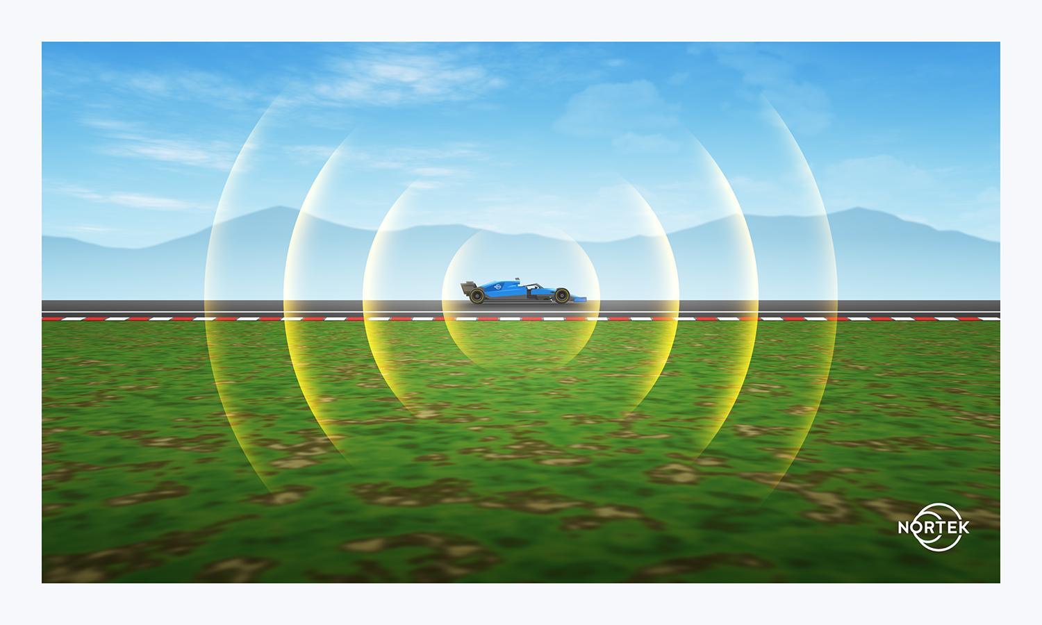
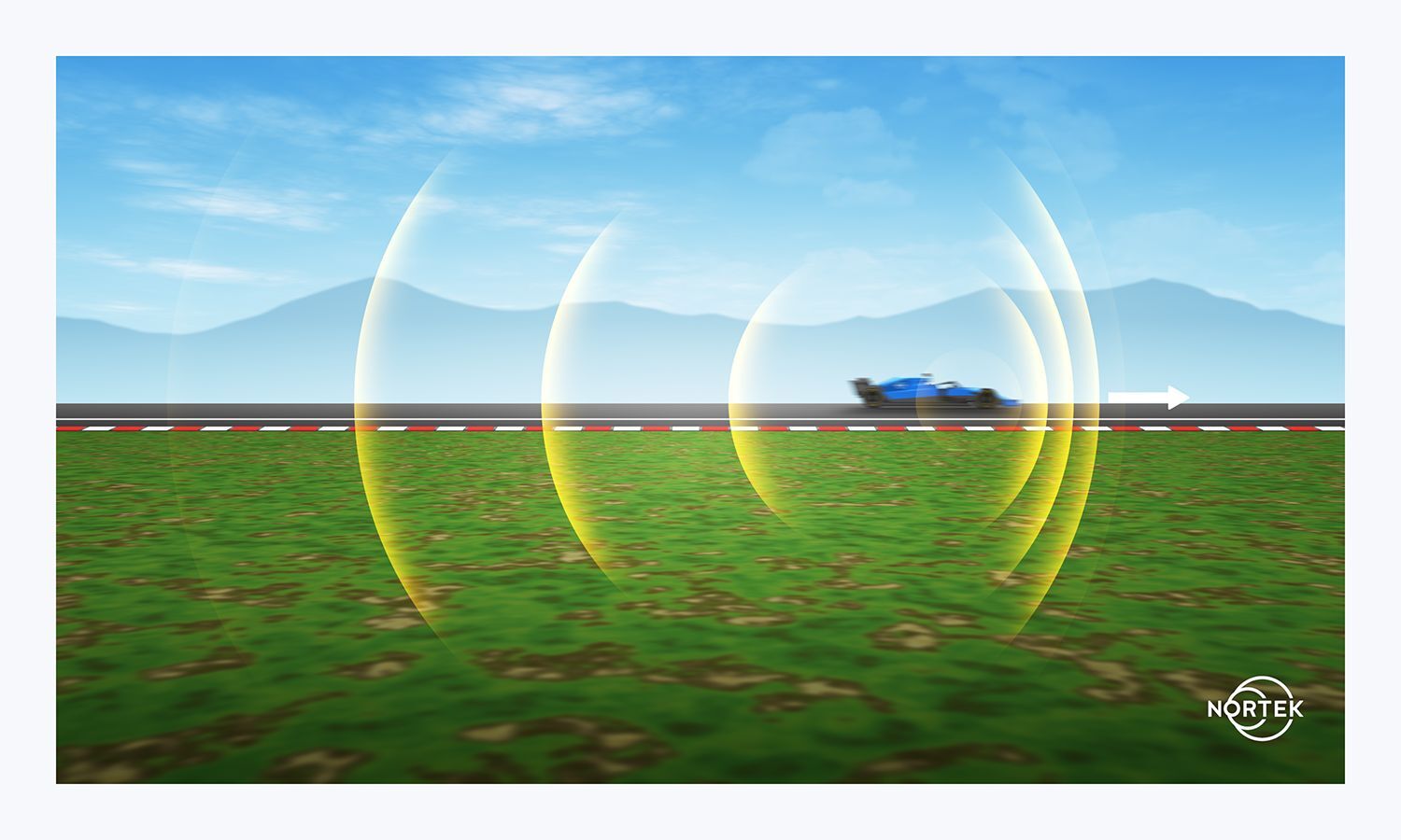
Figures 4A and 4B show why the car’s velocity changes the pitch of the sound of the engine. If you are standing beside a racetrack and a racing car goes by, the pitch of the sound coming from the car’s engine will change as it passes by you. This happens because the distance between you (the receiver) and the car (the source) is changing. When the car is approaching, the distance is decreasing and so the pitch increases, and vice versa. Although we’re using the sound of the engine in a racing car as an example, it can be any other source, such as the horn in a passenger car, as seen in this video:

The description below shows how to use the change in pitch of a car horn to compute the speed of the very same car.

When the car is approaching, the frequency of the horn is about 530 Hz, which falls to about 470 Hz as it leaves. The 60 Hz difference is double the Doppler frequency shift, Fd, because you hear the shift coming and again going (but shifting in the opposite direction). The frequency F of the horn when the car is standing still is the average of the two frequencies, i.e. 500 Hz.

The equation for the speed of the car is:

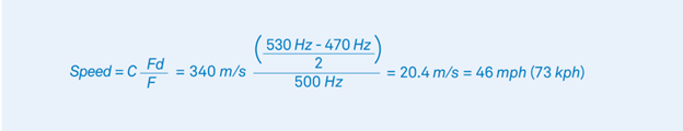
where C is the speed of sound in air.

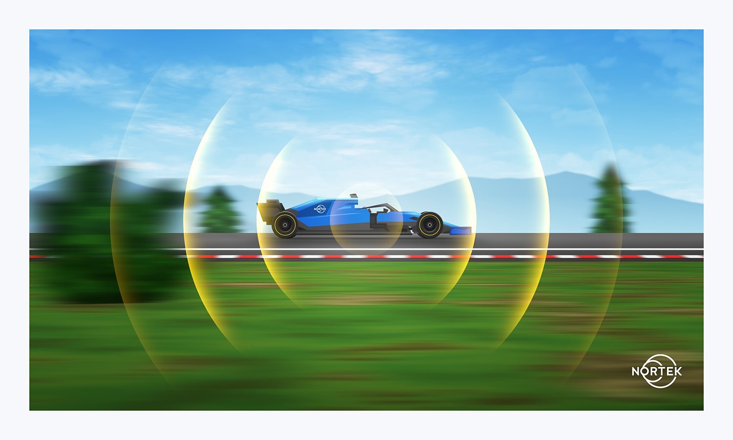
The apparent change in pitch (change in frequency, i.e. Doppler effect) is clearly observed in the above video. However, for the driver of the car, the pitch does not change, because he is moving with the car and so the distance between him and the horn does not change, and therefore there is no Doppler effect. A similar point is visualized in Figure 5, demonstrating how the Doppler effect requires relative motion between the source and receiver.

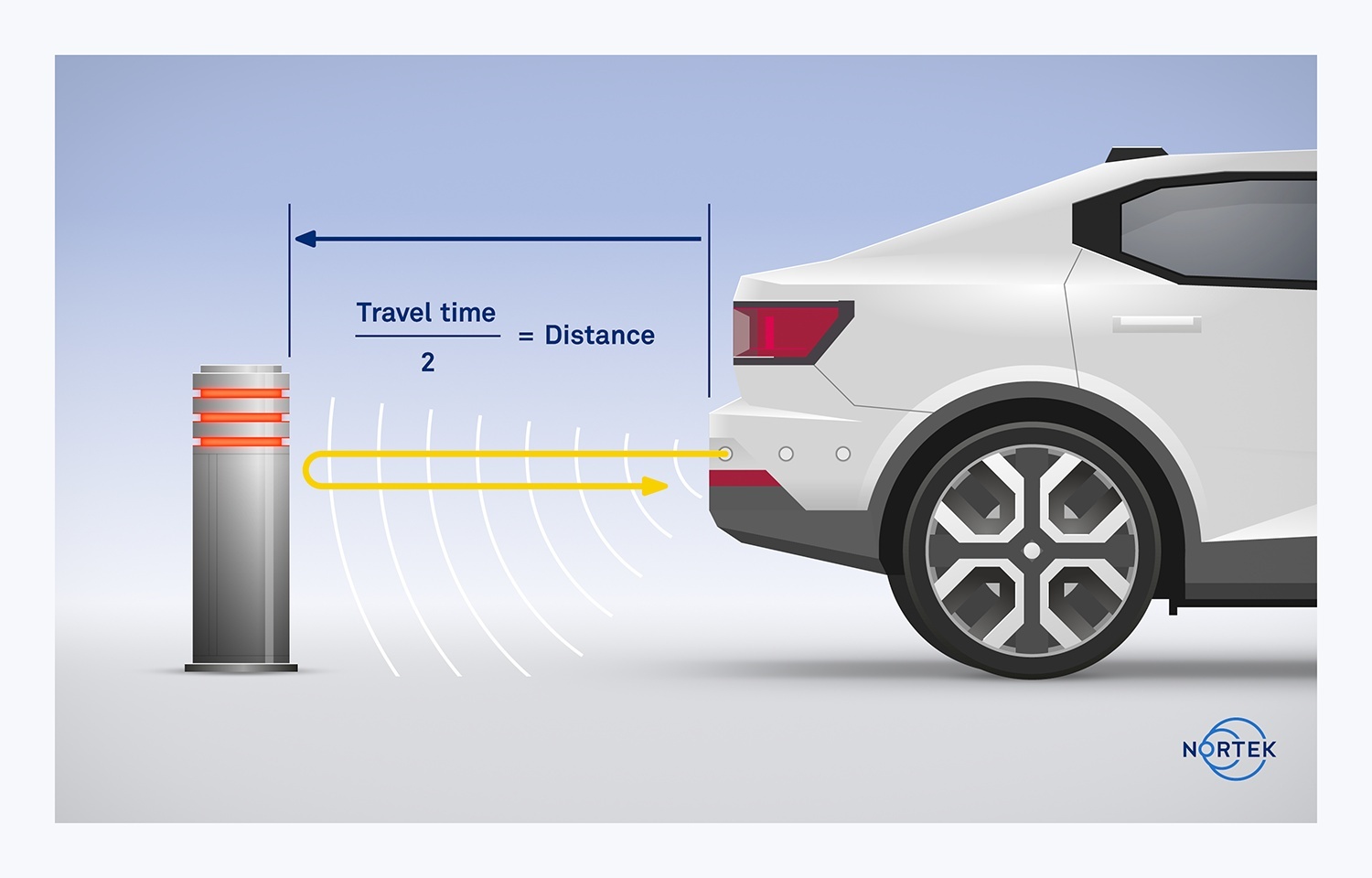
In addition to changes in frequencies (i.e. pitch), the Doppler effect can also be understood in terms of how it changes travel time. Consider the parking sensors in cars, the little sonars that listen for echoes of the sound pulses they send out. The time it takes for the pulses to travel to the obstacle and return to the sonar (the “two-way travel time”) tells the sonar how far away the obstacle is. As the car gets closer to the obstacle, the warning sound changes to alert the driver that the car is approaching an obstacle. The change in travel time of the sound pulses measures the car’s velocity, which is another way to use the Doppler effect.

3. How ADCPs use the Doppler effect

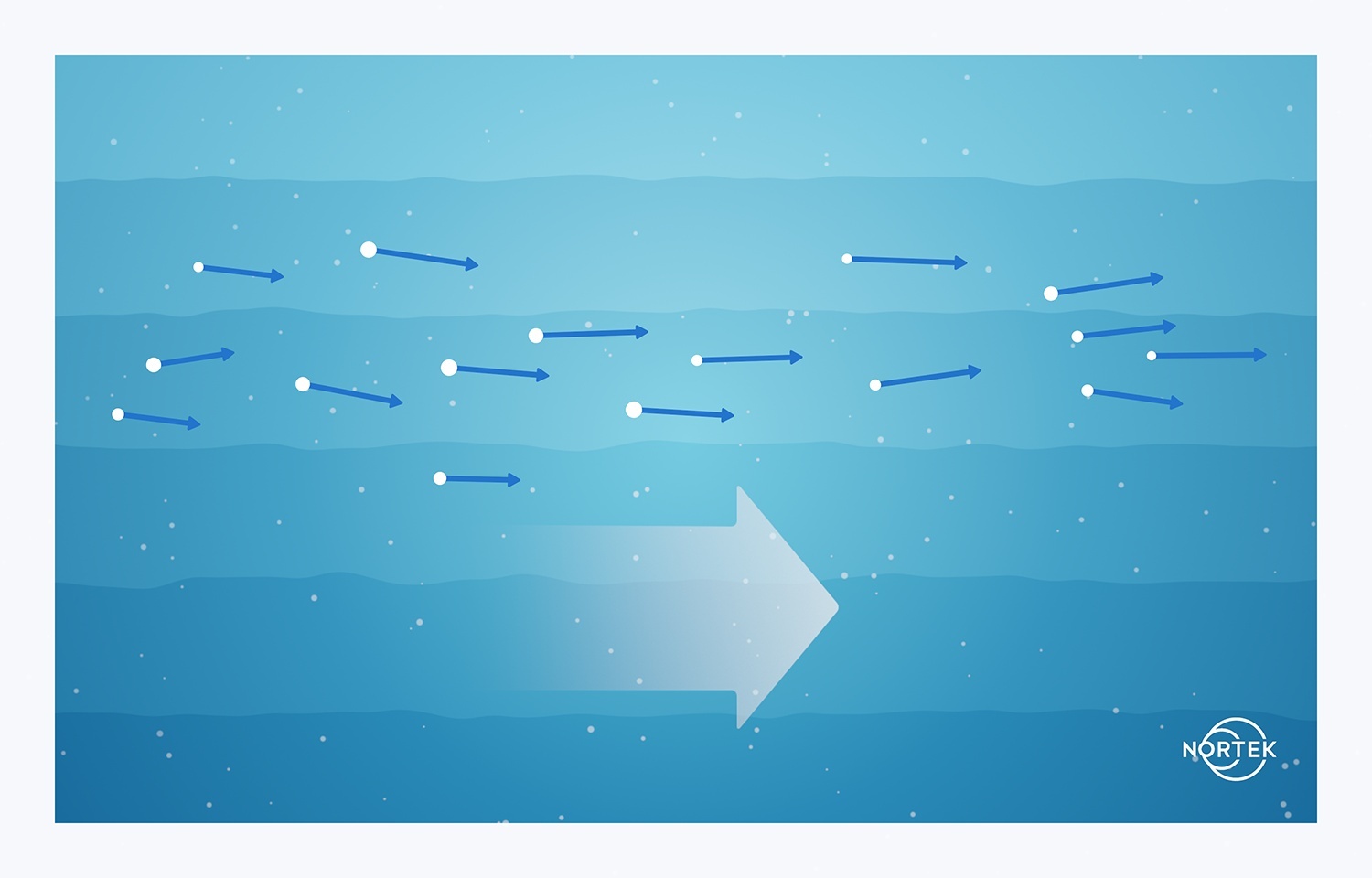
ADCPs actually measure water velocity indirectly by measuring the velocity of particles that are moving with the water. These particles are often zooplankton but may also be suspended sediment or other particles (Figure 7). ADCPs assume that the particles are moving at the same velocity as the water. This is nearly always a safe assumption, which is why the entire ADCP industry exists today. These particles are called scatterers, because they scatter (or deflect) the sound waves.

ADCPs measure the particles’ velocity using narrow beams of sound. They transmit (or send out) the sound, wait a short time, and listen for echoes from the particles. Doppler processing tells ADCPs how fast the particles are moving, and therefore the velocity of the water. ADCPs do this using acoustic frequencies that are too high for us to hear.

ADCPs can only sense the motion of particles that change their distance from the ADCP, which means that an ADCP beam can only detect motion that is parallel to that beam. Each beam measures a single component of the velocity, i.e. a one-dimensional (1D) velocity.

ADCPs that look up towards the water surface or down towards the sea bottom get 3D velocity profiles by using multiple slanted beams, with each beam pointing in a different direction. This requires assuming that the flow is “horizontally homogeneous” – that is, at a given depth, the velocity is the same in all the beams. Given the short distances between the ADCP beams, this is nearly always a good assumption.

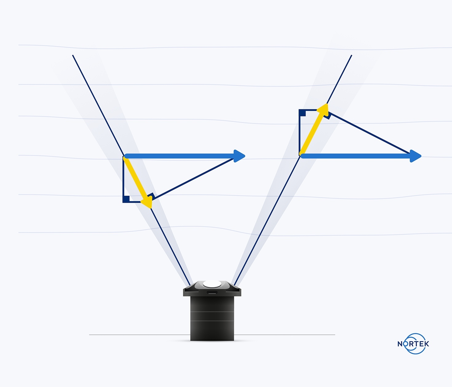
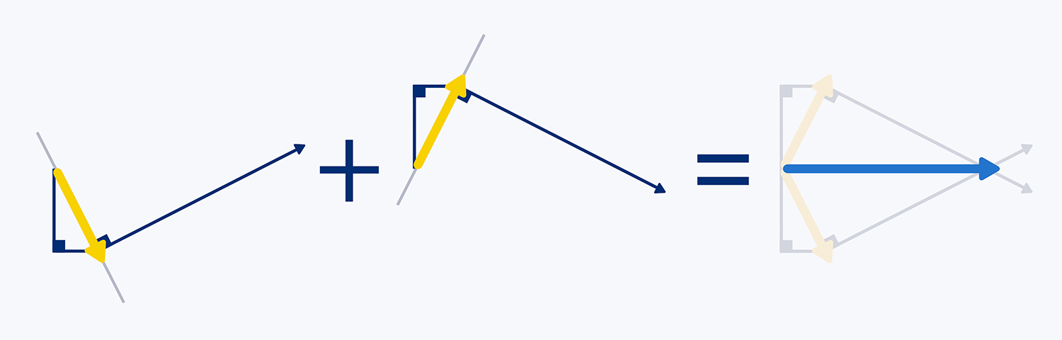
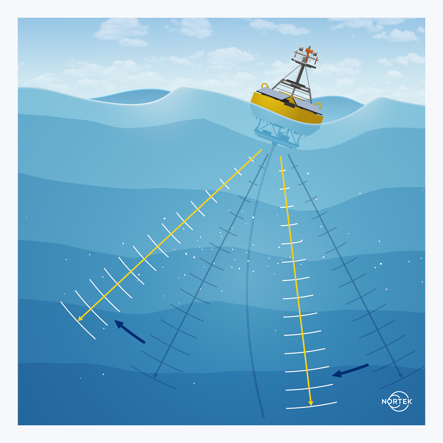
Figure 8 shows what two opposing beams see from an ADCP looking up. The actual water velocity (blue arrows) is the same for each beam, but each beam sees the velocity differently. The projection of the water velocity on the beam at the right produces a velocity away from the ADCP (yellow arrows). On the left, the projection is toward the ADCP. Figure 9 shows that the simple vector addition of the two beam-velocity vectors produces a result that is proportional to the horizontal water velocity. An ADCP with a left–right pair of beams will also have a front–back pair, and the combination of the two pairs of beams measures the horizontal velocity vector. The ADCP uses similar math to determine the vertical velocity, and now it has the full 3D velocity. Most of the time, the vertical velocity is much smaller than the horizontal. In fact, overall vertical velocity in the oceans averages out to zero.

The above description uses four beams to illustrate how ADCPs calculate 3D velocity, but three beams work just as well. The math changes a bit, but the result is the same.

The scale factor used to convert the ADCP measurement to actual water velocity depends on the ADCP’s beam geometry, and it is loaded into the ADCP when it is manufactured. The example given in Figures 8 and 9 assumes three conditions: 1) that the vertical water velocity is zero, 2) that the ADCP is perfectly level, and 3) that the ADCP is perpendicular to the flow. But the math works just as well when these conditions are not met. The process ADCPs use to correct data when the ADCP is not level and/or perpendicular to the flow is explained later in this guide.

4. Different Doppler processing techniques

ADCPs can measure water velocity through various methods, each with its own advantages and disadvantages. The two most common methods used in commercial ADCPs are generally called broadband and narrowband. The “band” in broadband and narrowband refers to the bandwidth of the acoustic pulse used. Finally, a third method is called Pulse-to-Pulse Coherent (or simply Pulse Coherent), which allows for very high temporal and spatial resolutions at the expense of range.

This section begins with basic broadband (or “wideband”) processing because narrowband is just a special case of broadband. There are different ways of implementing broadband in an ADCP. The simplest broadband implementation uses two short pulses of sound. The two pulses must reflect from the same scattering particles in order to get the particle’s velocity. This means the ADCP cannot wait very long between sending the first pulse and sending the second pulse. As a result, ADCPs normally put both pulses in the water at the same time. That is, in most broadband implementations, the ADCP does not wait for the first pulse to return to the ADCP before sending the second pulse.

We often call the scatterers in water “cloud scatterers” because they are distributed randomly, like the water droplets in a cloud. Each time the sound moves the length of its pulse, it returns echoes from new particles, which produces another independent estimate of the water velocity. Shorter pulses, commonly used in broadband, provide more independent estimates, which produces finer detail or improves the result by reducing random errors.

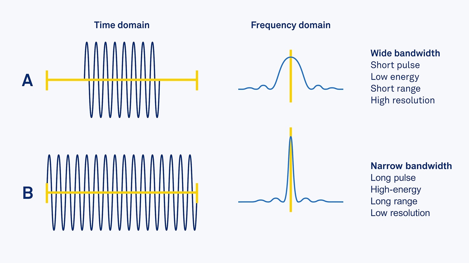
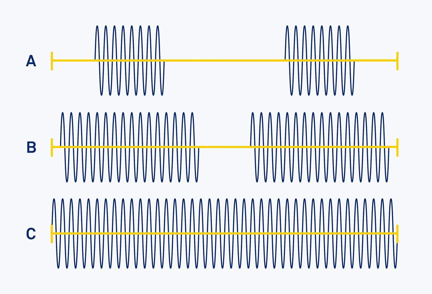
Bandwidth depends on the pulse length: the short pulses that give the best resolution also have the largest bandwidth. Figure 10 shows that bandwidth is inversely related to pulse length. In contrast, an unending pure tone has zero bandwidth and is often called a line spectrum. Broadband ADCPs use considerably shorter pulses than narrowband ADCPs, and they measure water velocity with considerably better temporal resolution.

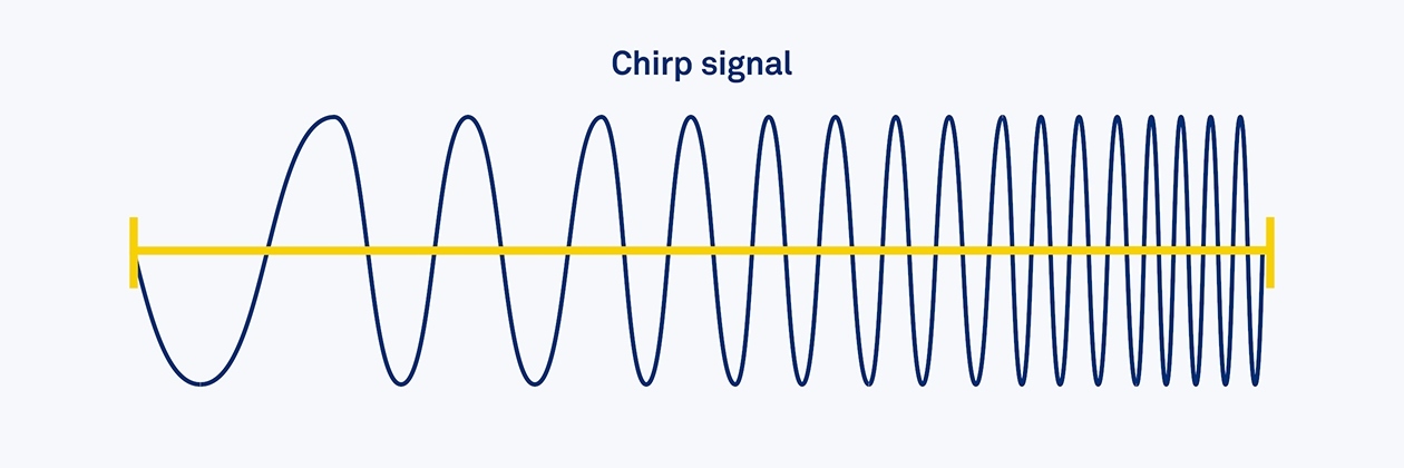
The problem with the short pulses typically used in broadband processing is that they do not get as much energy into the water as long pulses, and as a result, they cannot profile as far. The solution is to devise long pulses that have the bandwidth of a short pulse. Long pulses get more energy into the water and provide longer profiling ranges. If the signals maintain the short bandwidth, then the echoes can still be processed to get high-resolution water velocity data. One way to do this is to supplement the original two short pulses used in broadband with more of the same short pulses, except that some of them have their phase reversed (like flipping them upside down). Doing this allows the ADCP to differentiate between the pulses. Another broadband implementation uses chirps, where the pulse starts at one frequency and ends up at another, either higher or lower.

Returning to the original example of a broadband transmission consisting of just two short pure-tone pulses, imagine that the two short pulses progressively increase in length until the two just touch each other. This is illustrated in Figure 13. When this happens, the broadband transmission has become narrowband. A narrowband pulse can be treated as a special case of broadband with signal processing that is fundamentally the same. And narrowband is where ADCPs started, partly because it seemed conceptually simpler, but also because the microprocessors of that era had limited processing power. Broadband processing is more computationally intensive, but of course microprocessors are faster now.

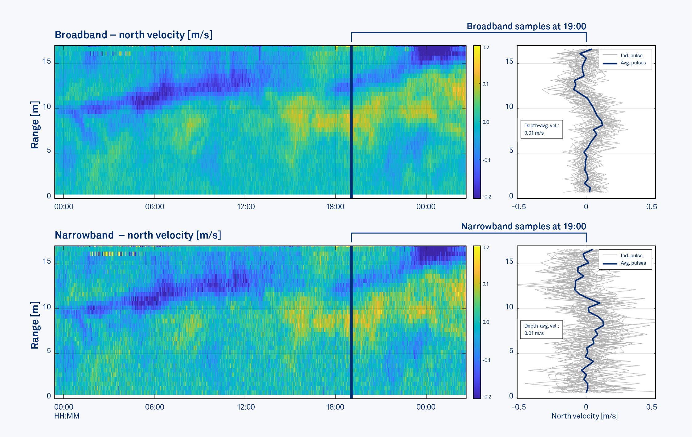
Earlier we said that broadband ADCPs capture finer details because their shorter pulses produce more independent estimates. This is illustrated in Figure 12, where an ADCP was set up to profile currents using both narrowband and broadband, alternating between the two methods every 60 seconds. Both methods captured well the general structures in the flow, and both gave the same depth-averaged velocity.

However, as shown in the contour plots on the left-hand side of the figure, the broadband method (top left) provides a greater level of detail than the narrowband method (bottom left).

Another reason broadband ADCPs obtain better detail is that they have more flexibility to separate sequential pulses. Greater pulse separation reduces measurement uncertainty, provided that they still see the same scatterers. This is also illustrated in Figure 12, where on the right-hand side we show the current profiles for 30 individual broadband pulses (top right) and 30 individual narrowband pulses (bottom right). It’s clear to see how the variability between individual pulses is smaller for broadband than narrowband. So, even though both methods provide the same depth-averaged velocity, broadband provides a greater level of detail.

While greater pulse separation allows broadband to provide us more detailed data, waiting too long can cause signal processing problems too (e.g. it affects the range of velocities the instrument can measure), so broadband ADCPs demand more care than narrowband ADCPs when setting them up for measurements.

Lastly, in addition to broadband and narrowband, we have a third Doppler processing method, called Pulse Coherent. In this processing method, a pair of pulses is transmitted, much like the broadband method; however, the pulses are separated by a relatively long distance such that the two pulses are not in the water at the same time. In the Pulse Coherent method, the intent is for the second pulse in the pulse pair to be transmitted only after the first pulse has been fully returned. The ADCP then calculates how similar the first pulse’s return signal is to the second pulse’s return signal and this value is directly proportional to the speed of the water. The Pulse Coherent method offers the best precision and time-space resolution of any Doppler technique by far, so it is perfect for fine-scale turbulence measurements. However, it is only capable of measuring relatively short distances (typically just a few meters) and low velocities (typically a few cm/s).

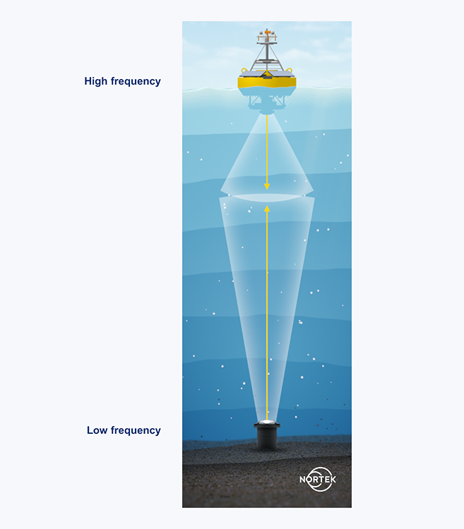
5. ADCP frequency and profiling range

Because ADCP bandwidth is proportional to frequency, high-frequency ADCPs have more bandwidth with which to obtain data with higher resolution. On the other hand, low-frequency ADCPs profile farther.

If profiling range is important to you, there are a few things you can do to increase the range. Some instruments allow you to adjust the transmit power, and more power brings you more range. Increasing the cell size has the same effect. For example, doubling the transmit pulse duration (often achieved by doubling the cell size; see Section 6) increases the energy transmitted by a factor of two, or 3 dB. However, acoustic attenuation is exponential, so doubling the power generally increases range by only a few percent.

In some places, for example in deep water far below the ocean surface, there are fewer scatterers and so echoes are weaker. Having fewer scatterers in the water reduces the ADCP’s range. If you moor an ADCP in the deep ocean, looking up, it will profile through the region of scatterers where its signal-to-noise ratio is strongest (because the signal is closer to the ADCP), and then it will have more scatterers at the end of its range where the signal-to-noise ratio is normally the weakest.

This approach produces the longest profiling range for an ADCP, and this is why in the open ocean, an up-looking ADCP will generally profile farther than a down-looking ADCP covering the same region. The drawback is that a deep ADCP loses data near the surface. If near-surface data is important to you, one option is to use an additional higher-frequency ADCP near the surface to get that data too.

6. ADCP range cells

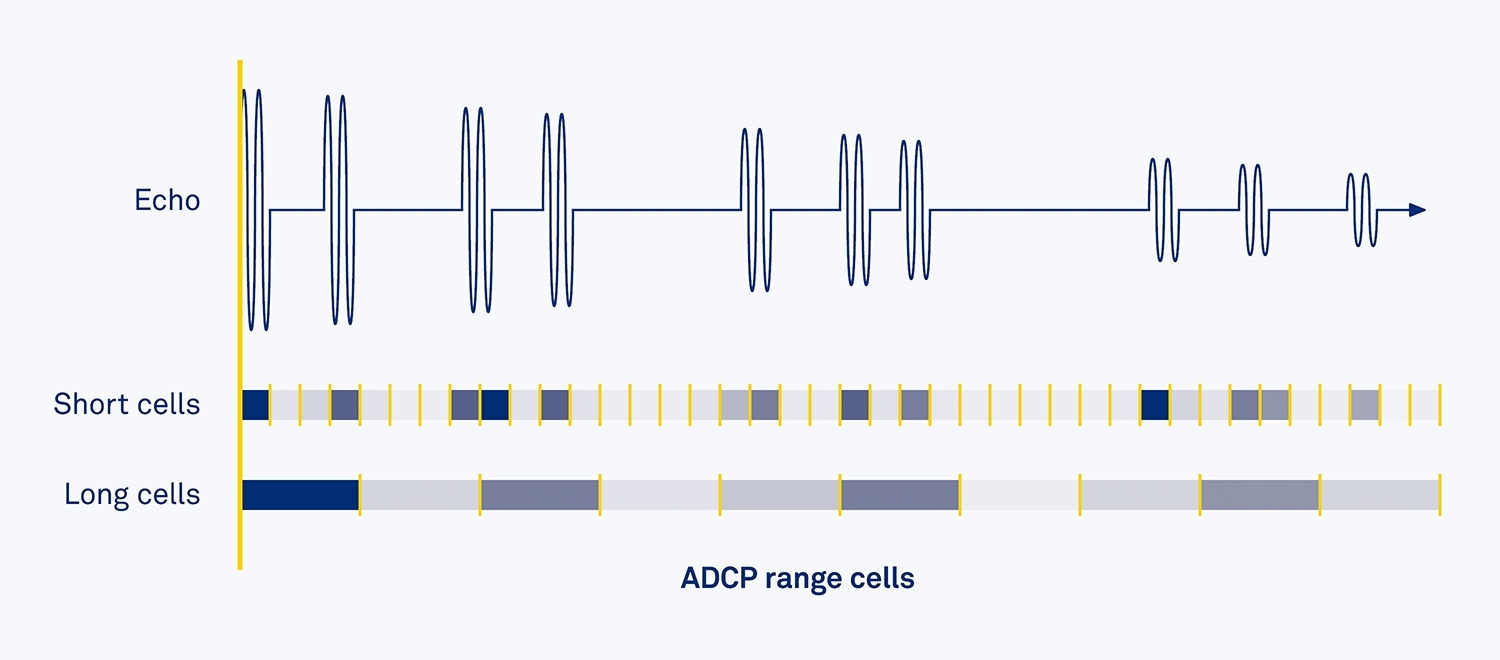
ADCPs divide their measurement profiles into segments called “range cells” or “bins”. The first echoes that return to the ADCP are from the first range cell. Echoes from the second range cell come back a moment later. Data return from cell after cell until the signal dies out and the ADCP can no longer calculate the velocity (see Figure 17).

ADCP depth cell size affects the profiling range, as we saw above, and also the velocity variance. The standard deviation, which is the square root of the variance, is the nominal size of the random errors in the data. A single ADCP measurement is called a ping, and ADCPs average a collection of pings to reduce the velocity variance.

Users can adjust the size of the ADCP range cells, but once set, the cell size is the same across the entire profile (with some rare exceptions). Shorter cells produce finer spatial detail, but at the cost of increased velocity variance. Averaging a collection of pings reduces variance, but this comes at the cost of temporal resolution (see Figure 18). The point of this is that selecting the cell size requires tradeoffs involving spatial resolution, temporal resolution and velocity variance.

Profiling ADCPs measure data in many cells over the profiling range, but there are other beam geometries too. Some current meters use two horizontal beams to measure the horizontal velocity at just a single depth. These current meters use a third, slanted beam to measure three-dimensional currents.

7. How the surface or bottom affects ADCP data

ADCP beams are sometimes called pencil beams because they are narrow. However, the beams are actually shaped like cones, not pencils, and they also leak sound out toward the sides. ADCP beams are like a flashlight or torch that is blinding when it points straight at you, but still visible when it points away.

The center of the beam is called the main lobe, which is the part of the beam that does the work for an ADCP. The leakage to the side is in sidelobes, and over most of an ADCP’s range the sidelobes have little effect on the ADCP’s measurements. This is because the main lobe carries most of the acoustic power. However, sound scatterers in the ocean reflect sound poorly compared with hard reflectors like the sea bottom or surface. Even though sidelobes are weak, sidelobe reflections from these surfaces are usually strong enough to introduce errors into the measurements.

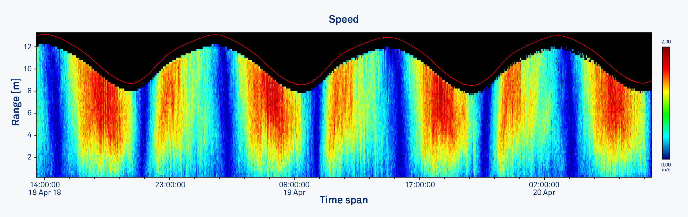
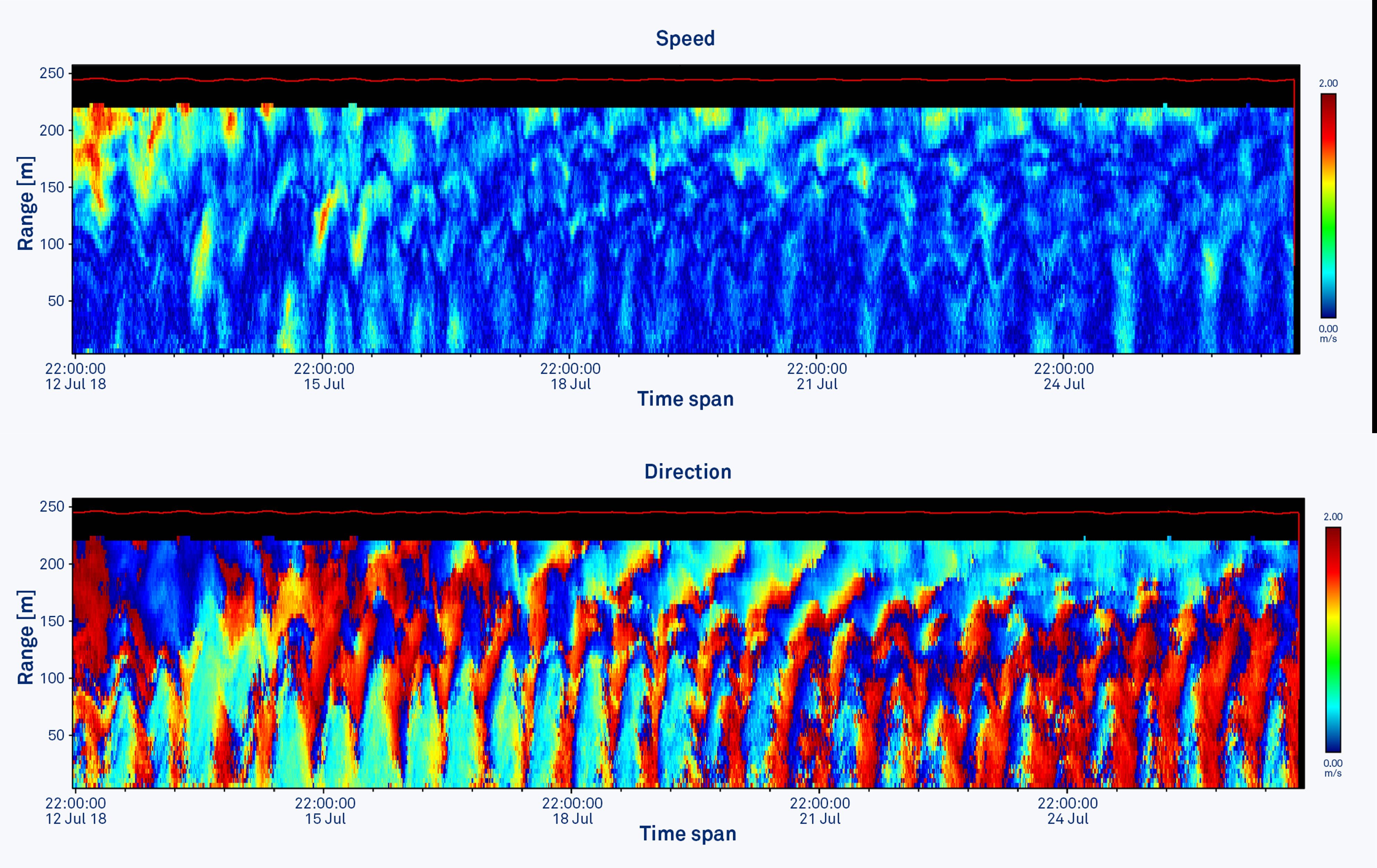
Since the surface and bottom are stationary on average (i.e. the vertical velocity is zero on average), sidelobe interference contaminates your velocity data by biasing it towards zero. Sidelobe interference produces stripes in color contour velocity plots at the sidelobe depth.

Sidelobes can also contaminate data when there are nearby reflective objects. For example, ADCPs mounted inline on a cable may have other sensors mounted on the cable in front of the beams. These sensors sometimes contaminate velocity data, just like echoes from the surface or bottom.

The reason it works this way is that, even though sidelobes are weak, the surface and many subsurface objects reflect sound better than the particles in the water (e.g. zooplankton). While sidelobes that point straight up are much weaker than the sound along the slanted main beam, the surface is such a strong reflector that the echoes from the surface can be as strong as the echoes in the main beam.

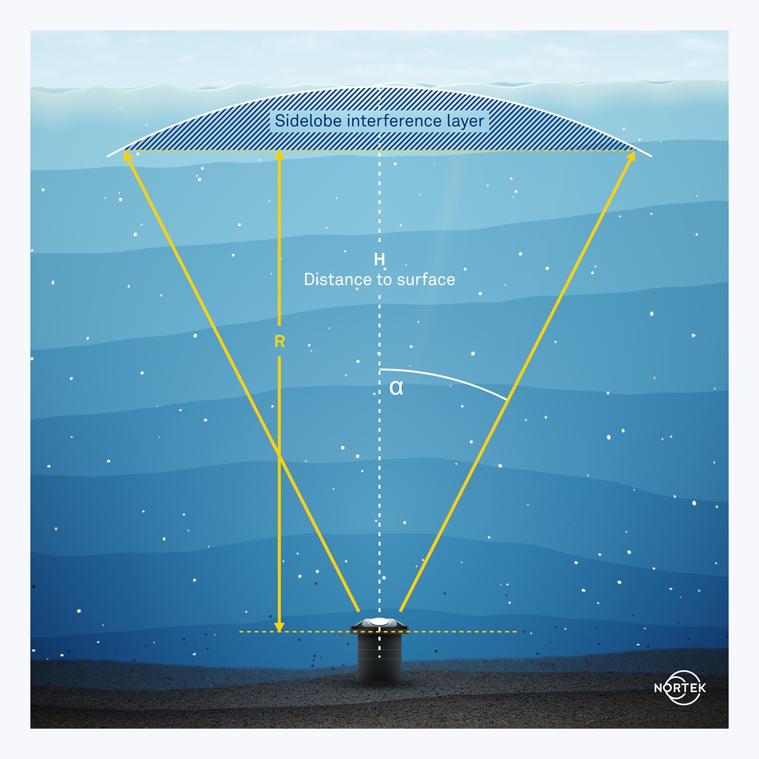
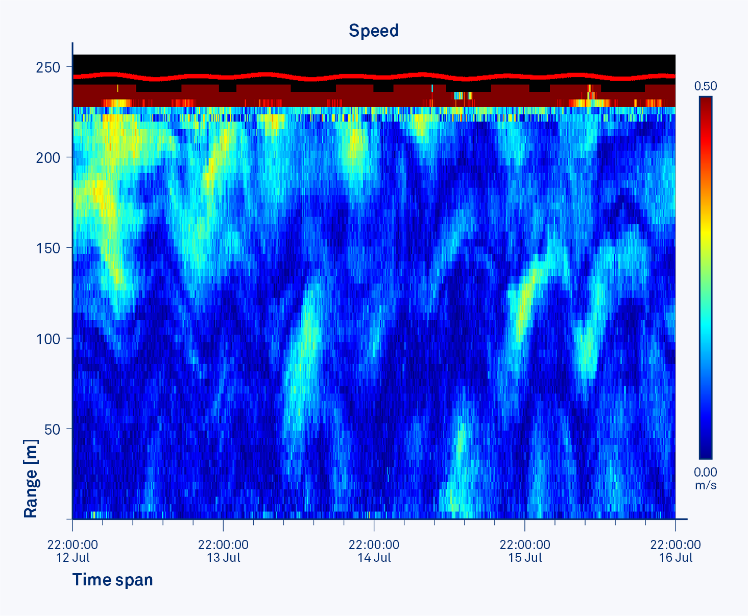
Figures 19 and 20 show where the sidelobes interfere with the velocity measurement. The depth of the interference depends on the slant angle of the beams. A slant angle of 30° gets good data to around 86% of the distance to the surface. Reducing the angle to 20° gets data to around 94% of the distance to the surface. The smaller slant angle gets closer, but at a cost of higher velocity standard deviation because the beam is more perpendicular to the flow than, say, a 30° slant angle. A 20° slant angle produces data with around double the variance of a 30° slant angle.

8. ADCPs and ringing

Early ADCPs had to allow their transducers to “ring down” before they could get good data because the transducers would continue to vibrate even after energy was transmitted. This meant ignoring data close to the ADCP that would have been biased by this ringing. Ringing was caused by the transducers and the transmit circuitry.

ADCPs are much better now. (The problem is smaller, but we still operate with the term blanking distance, which is just another way of describing ringing.) However, when you collect data close to the ADCP transducer, be alert for flow disturbances caused by the ADCP itself.

9. How an ADCP uses sound speed data

An ADCP uses the temperature at its transducer to calculate sound speed. ADCPs in deep water, e.g. > 1000 m, may also use the depth to compute sound speed. ADCPs need the sound speed to compute water velocity. Accurate sound velocity is important because an error in sound velocity produces a proportional error in its water velocity measurement.

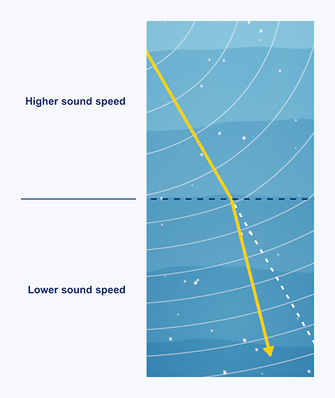
Sound velocity usually varies with the depth below the water surface, but the good news is that this variation has no effect on the horizontal ADCP’s velocity measurement. The reason for this is Snell’s law. Figure 21 shows that, as sound velocity changes across the layers of the ocean, continuity keeps the sound’s horizontal velocity component the same. Since the ADCP’s horizontal velocity measurement depends only on the sound’s horizontal velocity, the varying sound velocity has no effect on the ADCP’s velocity measurement.

An ADCP also uses sound speed to convert travel time into a distance to each depth cell. Since ADCPs know their beam geometry and their tilts (see section 10), they can convert the distance along the beam to the depth of each cell. They assume the sound speed is constant with depth, but if you know how temperature and salinity vary with depth, it is straightforward to correct cell depth for sound speed variations.

Sound speed depends on temperature, salinity and pressure, but the temperature has the greatest influence, hence ADCPs always have embedded temperature sensors. The speed of sound in water increases with increasing water temperature, increasing salinity and increasing depth. In typical ocean environments, sound speed varies by up to a few percent over the profiling range of an ADCP.

10. ADCP tilt sensors

ADCPs need to know their tilt so they can determine where their beams are and which way they are pointing. ADCPs need to know the exact angles of the beams to compute accurate velocity. Also, when depth cells on one beam tilt lower, the matching cells on the opposing beam go higher, and they see velocities at different depths. Some ADCPs use a mapping process to match the cells that are closest to a given level to compute velocity at that level.

ADCP beam angles are controlled with high precision during the manufacturing process. Standard ADCPs have three or four beams, all slanted the same and generally distributed uniformly around the instrument. Some profilers have beams pointing in a variety of angles. These angles are hard coded into the instrument, and ADCPs automatically account for them when they compute velocity.

However, when deployed, ADCPs can move around, both tilting and rotating (Figure 22). ADCPs handle this motion with sensors that measure tilt and heading.

A glass of wine illustrates how tilt sensors work. No matter how the glass tilts, gravity keeps the surface of the wine level. Modern tilt sensors use gravity in much the same way, and they are vastly better, smaller and less expensive than they were when ADCPs were first introduced.

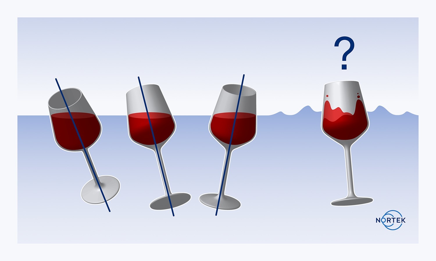
Just as the unsteady wine glass in Figure 23 would have trouble with tilt, horizontal accelerations introduce errors into ADCP tilt measurements. Surface waves are perhaps the most common cause of acceleration, but ADCPs mounted on strumming mooring lines in high currents can also experience accelerations. Both accelerations and tilt errors produce velocity errors in the ADCP data.

In most situations, accelerations have little effect on an ADCP’s overall measurement accuracy. Accelerations produce small velocity errors relative to normal measurement uncertainties, and they average out.

Tilt errors caused by accelerations cause the ADCP to miscalculate both its tilts and range cell location within the water column, but as the depth errors are approximately symmetric, one cell going positive and the other negative, they largely cancel each other out. The net result is some smearing of the vertical profile over depth.

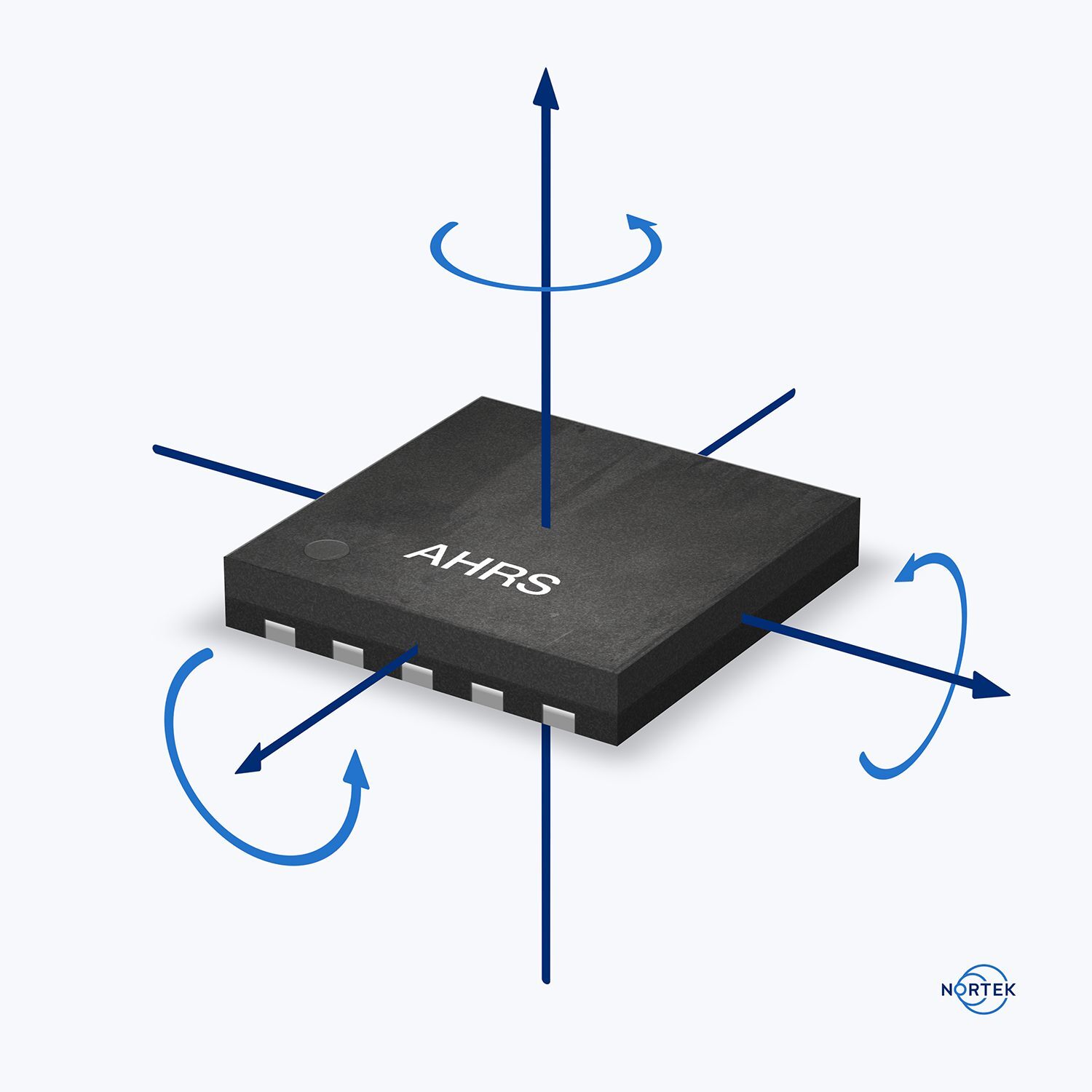
Some environments (particularly surface buoys) are so active that they introduce significant errors into ADCP data. Relatively recent technology enables ADCPs to eliminate these errors by measuring all components of the motion to enable an ADCP to accurately correct its data. Some ADCPs can add an Attitude and Heading Reference System (AHRS) that measures linear (i.e. back and forth, up and down) and rotational accelerations (Figure 24) as well as magnetometer data. A gyroscope in the AHRS enables the sensor to differentiate acceleration of the ADCP from the acceleration of gravity. An AHRS substantially improves the ADCP’s knowledge of its tilts, which in turn improves the ADCP’s data in active environments. An AHRS produces a lot of data, but modern processors have no trouble keeping up.

11. ADCP compasses

ADCPs must also know their heading in order to determine where their beams are pointed relative to north. In the past, ADCPs used many different kinds of compasses, but now, modern ADCPs mostly use magnetometers. Magnetometers measure three axes of the Earth’s magnetic field. The horizontal component provides the direction towards magnetic north.

Magnetic north is usually close to true north, and the difference is called the magnetic declination. The declination varies depending on where the ADCP is located on the Earth’s surface. You can look up the magnetic declination on a map or online and correct your data in post-processing.

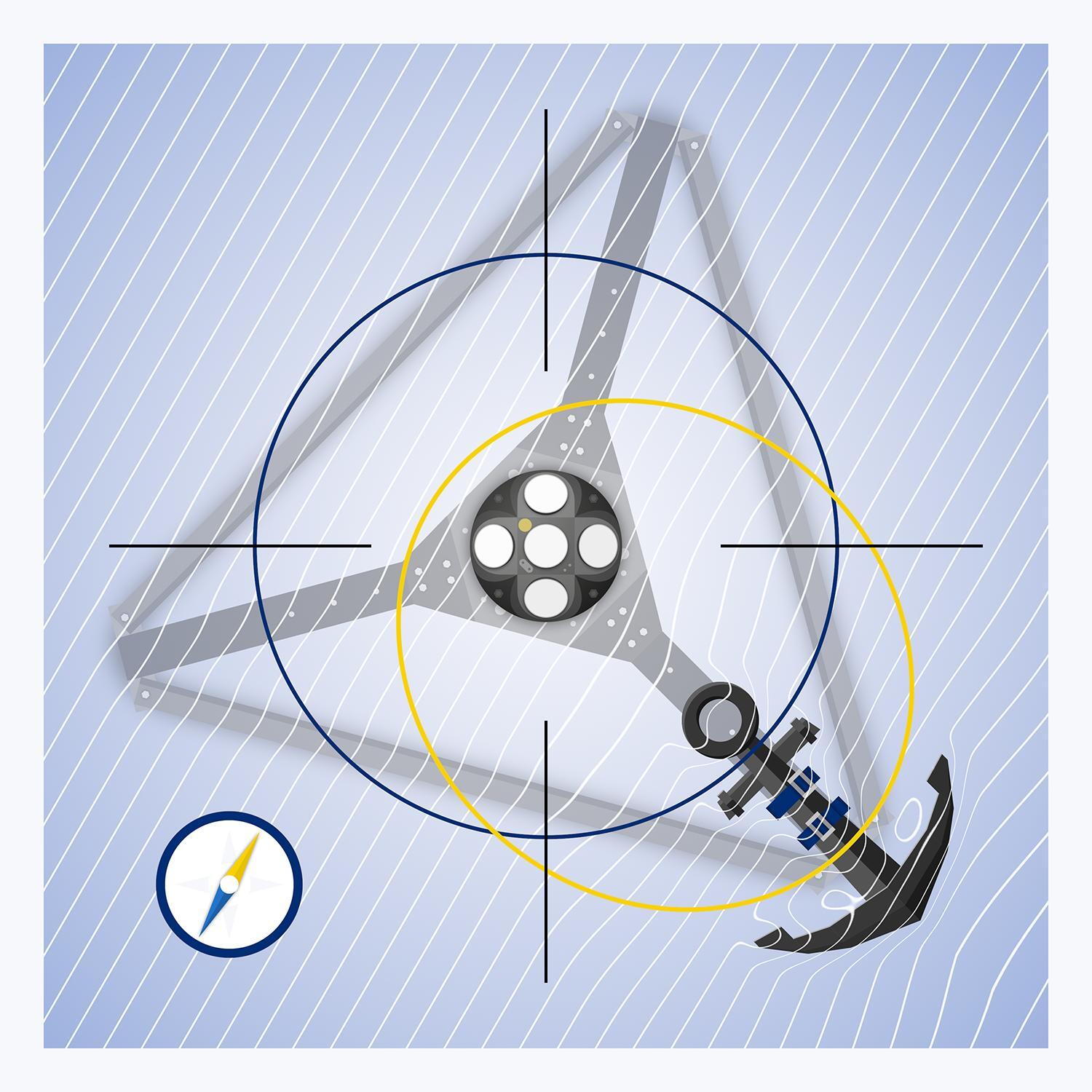
Magnetometer errors mostly arise from magnetic materials in the ADCP, its batteries, and its mount or frame. These offset and/or distort the Earth’s magnetic field, introducing errors in the heading measurement (see Figure 25). Compass calibration can correct for most of the errors, but not all of them if the interference is too strong.

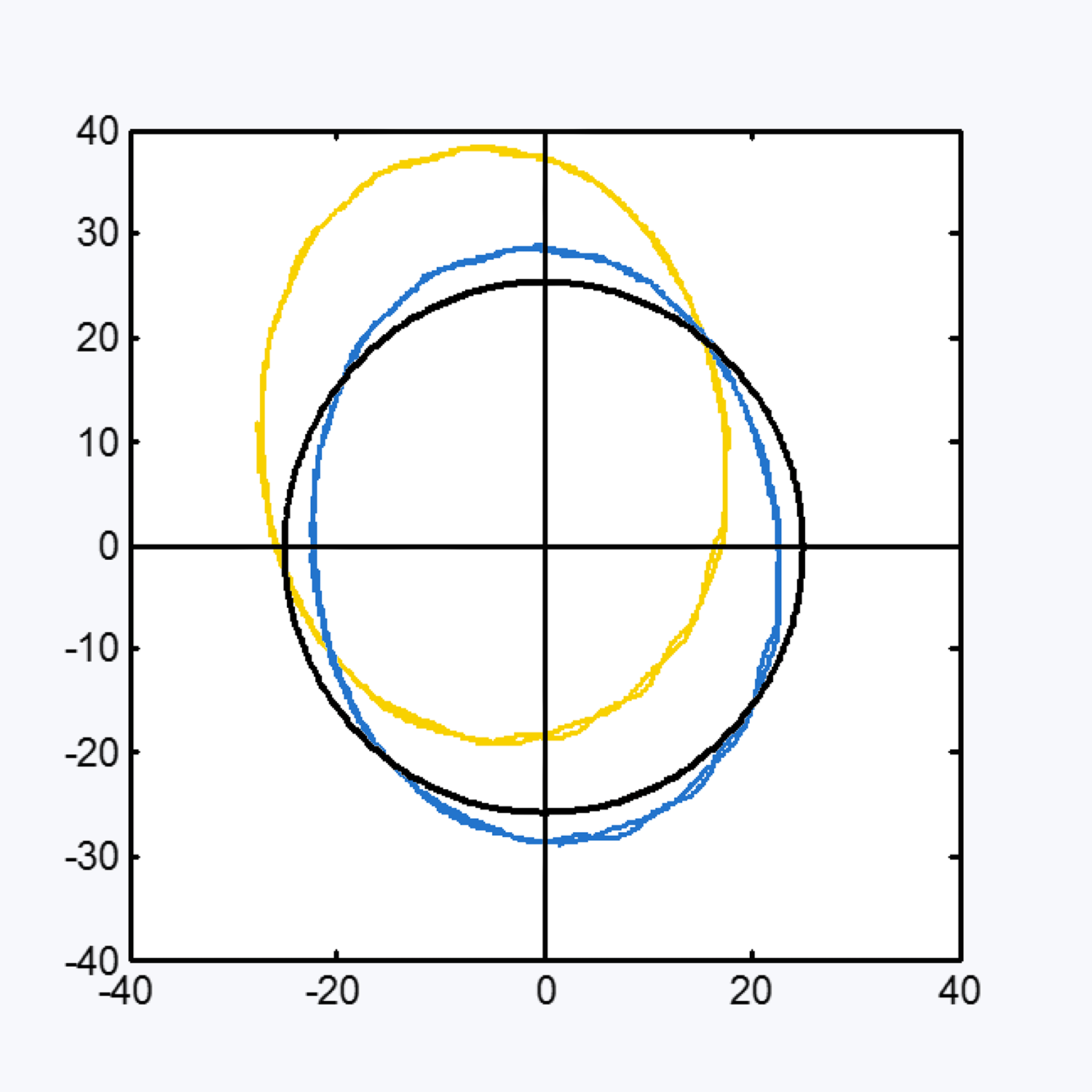
If a level, non-magnetic ADCP with a perfect magnetometer rotates as it measures the Earth’s magnetic field, a plot of the ADCP’s x- and y-axis magnetometer data would form a perfect circle centered on the origin (see black circle on Figure 26). The diameter of the circle is the horizontal magnitude of the Earth’s magnetic field at that location, and the angle provides the heading of the ADCP.

In practice, there is always nearby magnetic material, and this material introduces two classes of errors: “hard iron” and “soft iron” errors. The calibration in Figure 26 illustrates these errors for an ADCP mounted close to a huge steel buoy. The hard iron errors offset the circle from the origin, and the soft iron errors squeeze the circle into an oval.

Most ADCPs provide compass calibration procedures that can be used during deployment preparation. If possible, the ADCP should be calibrated in its mount. Some ADCPs collect raw magnetometer data, such as those equipped with an AHRS. If these ADCPs are free to rotate when they are in the water, this data can be used to calibrate the compass as a part of the post-processing.

12. Averaging data to reduce random errors

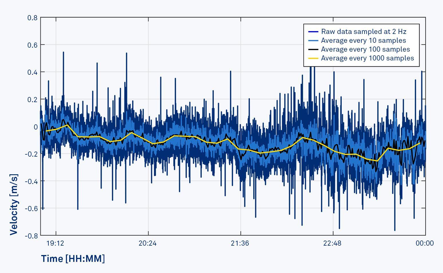
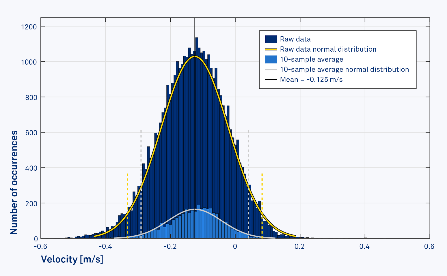
All ADCP data includes random errors. Figure 27 shows how random errors affect data, and how averaging may improve the data for some applications. The figure illustrates four separate time series taken from the same ADCP, which was set to ping continuously twice per second (2 Hz). The dark-blue line is the raw 2 Hz data. The light-blue line is the exact same data, but averaged over every ten samples. The black and yellow lines were averaged over 100 and 1000 samples, respectively. You’ll see how the variance in the blue line is noticeably larger than the others. Another way to show this is on Figure 28, where the raw data (in dark blue) is plotted as a histogram together with the data averaged over every ten samples (in light blue). The black vertical line is the mean of the data, which is the same for both cases. Fitted to these histograms are normal (Gaussian) distributions, and vertical dashed lines show the limits of two standard deviations on either side of the mean. Note how the standard deviation (which is the square root of the variance) for the raw data is wider than for the averaged data.

Averaging the data reduces the size of the random errors. The variance of the random errors decreases as the inverse of the number of data points averaged together (and the standard deviation decreases with the square root of the number averaged).

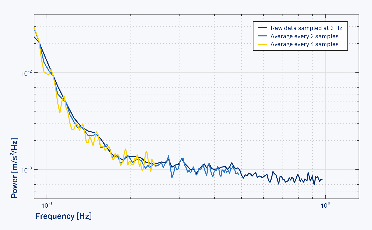
However, averaging doesn’t always improve your data. The quality of ADCP data has improved greatly since the advent of ADCPs, and when ADCP data is well above the minimal resolvable limit for the current in question, averaging does little other than remove (potentially) useful information. For example, in Figure 29 we show the same raw 2 Hz data plot in the frequency domain as a spectrum; that is, the amount of energy that is present at each frequency contained in the data. In this case, averaging these data simply removes the highest frequencies, which might actually be of interest (e.g. for turbulence studies). But don’t worry – for most applications, the instrument’s configuration software guides you through choosing an averaging interval that will meet your deployment’s requirements. And, if you are an advanced user who likes to work with the raw data, that is also possible.

13. Glossary

We realize that some of the terms in this glossary may have multiple meanings depending on their application or context (e.g. bandwidth or pulse), so unless otherwise noted, here the intended context is underwater acoustics as applicable to ADCPs.

• Accuracy
  • Numerical value expressing how close a measurement is to the true value. Accuracy may be expressed in terms of percentage (ratio between the measurement and the true value) or in the same units. Accuracy has two components, bias and standard deviation, both defined below.
• ADCP (Acoustic Doppler Current Profiler)
  • An instrument that measures a velocity profile in water by transmitting sound pulses of a given frequency and detecting the Doppler shift of the pulses as they reflect off particles in the water.
• Attenuation
  • The decrease in intensity of a given signal, typically as a function of distance away from the signal’s source. In underwater acoustics, attenuation can often follow a logarithmic decay curve. Higher-frequency acoustics has more attenuation than low-frequency acoustics, which is why low-frequency acoustics measures greater distances.
• Bandwidth
  • The difference between the lower and higher frequencies in a continuous spectrum, given as a percentage of the mean frequency. It is the inverse of pulse length.
• Beam
  • The narrow ray of acoustic energy emanating from the acoustic transducer of an ADCP.
• Bias
  • A systematic error in a set of measurements. For example, a scale that always measures 1 kg more than the actual weight. In ADCP measurements, bias often refers to the error in the measurement after the data has been averaged to remove random errors (noise).
• Broadband
  • Generic term for any ADCP whose transducer bandwidth is greater than about 12%.
• Chirp
  • An acoustic signal whose frequency either increases or decreases with time.

• Compass
  • An instrument capable of detecting the Earth’s magnetic field, thus providing magnetic heading information to the ADCP.
• Current meter
  • An instrument that measures water velocity within a single volume of water, as opposed to a profile.
• Cutoff
  • Generic term for a maximum or minimum threshold of a given value or parameter.
• Decibel
  • A unit of measurement for the power of an acoustic signal, expressed on a logarithmic scale and defined as the ratio of a measured quantity to a reference quantity. Symbol: dB.
• Depth cell
  • A single segment of a profile along a beam within which velocity is measured. The collection of depth cells at the same distance away from the ADCP forms a layer of a known thickness. Depth cells are often simply called cells, and they are sometimes called bins or range cells.
• Doppler effect
  • An apparent change in frequency when the sender is moving relative to the listener. An ADCP doubles the Doppler effect because it works between the ADCP and the reflectors in the water, and then again after the sound is reflected back to the ADCP.
• Doppler Velocity Log
  • Often abbreviated DVL, this is a special type of ADCP whose primary function is to measure an underwater vehicle’s speed and direction over the sea bottom.
• Down-looking
  • Said of an ADCP’s physical orientation when its transducers are pointing downward.
• Geometry
  • The specific and fixed arrangement for an ADCP’s transducers as it pertains to their inclination off the instrument’s vertical axis and angle of separation between transducers.
• Hard iron
  • A local magnetic distortion causing an ADCP’s compass to provide incorrect heading data. Hard iron errors produce a vector offset of the local magnetic field.
• Heading
  • The bearing along a compass rose that the ADCP is pointing, or that its velocity is referenced to.
• Hertz
  • Unit of measure for frequency, with units of cycles per second.
• Linear
  • Said of any measurement, parameter or function whose graphical representation is a straight line.
• Magnetic declination
  • The difference between magnetic north (where the compass needle points to) and geographical north (i.e. the North Pole).
• Magnetometer
  • An instrument that measures magnetic fields. An ADCP uses magnetometers to determine its heading.
• Main lobe
  • A cone-shaped region around the center line of an acoustic beam where most of the beam’s acoustic energy is concentrated.
• Narrowband
  • Generic term for any ADCP whose transducer bandwidth is less than about 12%.
• Phase
  • The angular difference between two periodic signals.
• Ping
  • Complete envelope of the acoustic signal emitted from a transducer; may contain pulses of a fixed frequency (monochromatic) or variable frequency (chirp). Often (incorrectly) used interchangeably with “pulse”.
• Pitch
  • Rotation about the ADCP’s y-axis.
• Precision
  • Numerical value expressing how close a set of independent measurements are to each other, expressed in the same units as the measurements themselves. Unlike accuracy, precision does not require knowledge of the actual (true) value.
• Profile
  • The combination of measurements from physically adjacent depth cells.
• Profiling range
  • The maximum distance an acoustic signal can reach.
• Pulse
  • The sound wave generated by an acoustic transducer.
• Pulse length
  • The extent of an acoustic pulse. Pulse length is often described in units of milliseconds (ms) as measured from the time the transducer is initially excited to the end of the excitation period. However, it can also be described in units of length given a known speed of sound.
• Pure tone
  • A pulse with a perfectly fixed frequency, often with a long duration.
• Receiver
  • The component responsible for detecting the reflected acoustic energy generated from a source. Can refer to the actual transducer on the ADCP or the electronic components responsible for collecting and initially conditioning the energy. For ADCPs, the same transducer is used to both transmit as well as receive the acoustic signal, whereas velocimeters have dedicated transmitting (source) and receiving elements.
• Reflector
  • Any particle, surface or region that reflects acoustic energy.
• Resolution
  • The detectable limit for a given parameter. For example, the spatial resolution of an ADCP is determined by the size of its smallest cell (e.g. 20 cm). Can also be applied to time (temporal resolution); for example, if an ADCP’s maximum sampling rate is 1 Hz, its best temporal resolution is 1 s.
• Roll
  • Rotation about the ADCP’s x-axis.
• Scatterer
  • Similar to reflector, but more commonly applied to particles alone.
• Sidelobe
  • While most of the energy in an acoustic beam runs through its main lobe, much weaker energy also leaks out at other angles in the sidelobes.
• Side-looking
  • Said of an ADCP’s physical orientation when its transducers are pointing horizontally.
• Signal-to-noise ratio
  • The strength of an acoustic signal compared with the instrument’s noise level. The measure is the log of the ratio of the two, expressed in units of decibels (dB).
• Soft iron
  • A local magnetic distortion causing an ADCP’s compass to provide incorrect heading data. Soft iron errors cause the measured magnitude of the local magnetic field to vary with the heading of the instrument. A perfect magnetometer measures a constant magnitude, no matter the heading.
• Source
  • The component responsible for transmitting acoustic energy. Can refer to the actual transducer on the ADCP or the location where the signal originates. For ADCPs, the same transducer is used to both transmit and to receive the acoustic signal, whereas velocimeters have a dedicated transmitter (source) and several receiving elements.
• Spectrum
  • The graphical representation of a signal in the frequency domain, where the signal’s energy is plotted as function of frequency.
  • The frequency distribution of a signal. The spectrum divides the energy of the signal into a range of frequency bands.
• Standard deviation
  • A statistical measure of the variability of a value A, defined by:

where µ is the mean of A. Note that S is the square root of the variance. Standard deviation is also called random error, with the understanding that it is the rough magnitude of the error of any given measurement, but that on average, the error is zero.

• Tilt
  • A measure of an ADCP’s inclination; that is, variation from vertical. Tilt includes both pitch and roll.
• Transducer
  • Any device that transforms energy from one form into another. ADCP transducers’ main element is a piezoelectric ceramic that transforms electrical current into an analog acoustic (pressure) wave, or the other way around. ADCP transducers can function as sources transmitting acoustic signals, or as receivers converting sound into electrical signals.
• Transmit power
  • A measure of the energy transmitted by an ADCP transducer. It can be expressed in terms of decibels (dB) or watts (W).
• Travel time
  • The time it takes for an acoustic pulse to move a given distance away from the transducer, for example the time required for the sound to get to a particular cell, or to the end of the profile. ADCPs use the “two-way” travel time because the sound must go out and then back again.
• Up-looking
  • Said of an ADCP’s physical orientation when its transducers are pointing upward.
• Vector
  • A mathematical quantity having both a magnitude and a direction. Also the name of a velocimeter manufactured by Nortek.
• Velocimeter
  • A water-velocity measuring device that, unlike ADCPs, uses a transmitter and several separate receivers, which allow it to focus on a single small volume of water. Velocimeters are able to sample at much higher rates than ADCPs (i.e. up to 200 Hz), and their errors are much smaller.
• Wavelength
  • The physical distance between two successive wave fronts of an acoustic signal.